The tutorial shows how to create multiple IF statements in Excel with AND as well as OR logic. Also, you will learn how to use IF together with other Excel functions.
In the first part of our Excel IF tutorial, we looked at how to construct a simple IF statement with one condition for text, numbers, dates, blanks and non-blanks. For powerful data analysis, however, you may often need to evaluate multiple conditions at a time. The below formula examples will show you the most effective ways to do this.
How to use IF function with multiple conditions
In essence, there are two types of the IF formula with multiple criteria based on the AND / OR logic. Consequently, in the logical test of your IF formula, you should use one of these functions:
- AND function - returns TRUE if all the conditions are met; FALSE otherwise.
- OR function - returns TRUE if any single condition is met; FALSE otherwise.
To better illustrate the point, let's investigate some real-life formulas examples.
Excel IF statement with multiple conditions (AND logic)
The generic formula of Excel IF with two or more conditions is this:
Translated into a human language, the formula says: If condition 1 is true AND condition 2 is true, return value_if_true; else return value_if_false.
Suppose you have a table listing the scores of two tests in columns B and C. To pass the final exam, a student must have both scores greater than 50.
For the logical test, you use the following AND statement: AND(B2>50, C2>50)
If both conditions are true, the formula will return "Pass"; if any condition is false - "Fail".
=IF(AND(B2>50, B2>50), "Pass", "Fail")
Easy, isn't it? The screenshot below proves that our Excel IF /AND formula works right:

In a similar manner, you can use the Excel IF function with multiple text conditions.
For instance, to output "Good" if both B2 and C2 are greater than 50, "Bad" otherwise, the formula is:
=IF(AND(B2="pass", C2="pass"), "Good!", "Bad")
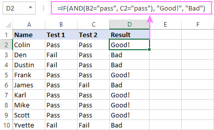
Important note! The AND function checks all the conditions, even if the already tested one(s) evaluated to FALSE. Such behavior is a bit unusual since in most of programming languages, subsequent conditions are not tested if any of the previous tests has returned FALSE.
In practice, a seemingly correct IF statement may result in an error because of this specificity. For example, the below formula would return #DIV/0! ("divide by zero" error) if cell A2 is equal to 0:
=IF(AND(A2<>0, (1/A2)>0.5),"Good", "Bad")
The avoid this, you should use a nested IF function:
=IF(A2<>0, IF((1/A2)>0.5, "Good", "Bad"), "Bad")
For more information, please see IF AND formula in Excel.
Excel IF function with multiple conditions (OR logic)
To do one thing if any condition is met, otherwise do something else, use this combination of the IF and OR functions:
The difference from the IF / AND formula discussed above is that Excel returns TRUE if any of the specified conditions is true.
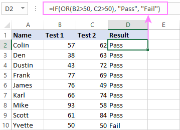
So, if in the previous formula, we use OR instead of AND:
=IF(OR(B2>50, B2>50), "Pass", "Fail")
Then anyone who has more than 50 points in either exam will get "Pass" in column D. With such conditions, our students have a better chance to pass the final exam (Yvette being particularly unlucky failing by just 1 point :)
Tip. In case you are creating a multiple IF statement with text and testing a value in one cell with the OR logic (i.e. a cell can be "this" or "that"), then you can build a more compact formula using an array constant.
For example, to mark a sale as "closed" if cell B2 is either "delivered" or "paid", the formula is:
=IF(OR(B2={"delivered", "paid"}), "Closed", "")
More formula examples can be found in Excel IF OR function.
IF with multiple AND & OR statements
If your task requires evaluating several sets of multiple conditions, you will have to utilize both AND & OR functions at a time.
In our sample table, suppose you have the following criteria for checking the exam results:
- Condition 1: exam1>50 and exam2>50
- Condition 2: exam1>40 and exam2>60
If either of the conditions is met, the final exam is deemed passed.
At first sight, the formula seems a little tricky, but in fact it is not! You just express each of the above conditions as an AND statement and nest them in the OR function (since it's not necessary to meet both conditions, either will suffice):
OR(AND(B2>50, C2>50), AND(B2>40, C2>60)
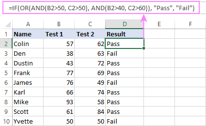
Then, use the OR function for the logical test of IF and supply the desired value_if_true and value_if_false values. As the result, you get the following IF formula with multiple AND / OR conditions:
=IF(OR(AND(B2>50, C2>50), AND(B2>40, C2>60), "Pass", "Fail")
The screenshot below indicates that we've done the formula right:
Naturally, you are not limited to using only two AND/OR functions in your IF formulas. You can use as many of them as your business logic requires, provided that:
- In Excel 2007 and higher, you have no more than 255 arguments, and the total length of the IF formula does not exceed 8,192 characters.
- In Excel 2003 and lower, there are no more than 30 arguments, and the total length of your IF formula does not exceed 1,024 characters.
Nested IF statement to check multiple logical tests
If you want to evaluate multiple logical tests within a single formula, then you can nest several functions one into another. Such functions are called nested IF functions. They prove particularly useful when you wish to return different values depending on the logical tests' results.
Here's a typical example: suppose you want to qualify the students' achievements as "Good", "Satisfactory" and "Poor" based on the following scores:
- Good: 60 or more (>=60)
- Satisfactory: between 40 and 60 (>40 and <60)
- Poor: 40 or less (<=40)
Before writing a formula, consider the order of functions you are going to nest. Excel will evaluate the logical tests in the order they appear in the formula. Once a condition evaluates to TRUE, the subsequent conditions are not tested, meaning the formula stops after the first TRUE result.
In our case, the functions are arranged from largest to smallest:
=IF(B2>=60, "Good", IF(B2>40, "Satisfactory", "Poor"))
Naturally, you can nest more functions if needed (up to 64 in modern versions).

For more information, please see How to use multiple nested IF statements in Excel.
Excel IF array formula with multiple conditions
Another way to get an Excel IF to test multiple conditions is by using an array formula.
To evaluate conditions with the AND logic, use the asterisk:
To test conditions with the OR logic, use the plus sign:
To complete an array formula correctly, press the Ctrl + Shift + Enter keys together. In Excel 365 and Excel 2021, this also works as a regular formula due to support for dynamic arrays.
For example, to get "Pass" if both B2 and C2 are greater than 50, the formula is:
=IF((B2>50) * (C2>50), "Pass", "Fail")

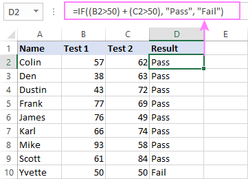
In my Excel 365, a normal formula works just fine (as you can see in the screenshots above). In Excel 2019 and lower, remember to make it an array formula by using the Ctrl + Shift + Enter shortcut.
To evaluate multiple conditions with the OR logic, the formula is:
=IF((B2>50) + (C2>50), "Pass", "Fail")
Using IF together with other functions
This section explains how to use IF in combination with other Excel functions and what benefits this gives to you.
Example 1. If #N/A error in VLOOKUP
When VLOOKUP or other lookup function cannot find something, it returns a #N/A error. To make your tables look nicer, you can return zero, blank, or specific text if #N/A. For this, use this generic formula:
For example:
If #N/A return 0:
If the lookup value in E1 is not found, the formula returns zero.
=IF(ISNA(VLOOKUP(E1, A2:B10, 2,FALSE )), 0, VLOOKUP(E1, A2:B10, 2, FALSE))
If #N/A return blank:
If the lookup value is not found, the formula returns nothing (an empty string).
=IF(ISNA(VLOOKUP(E1, A2:B10, 2,FALSE )), "", VLOOKUP(E1, A2:B10, 2, FALSE))
If #N/A return certain text:
If the lookup value is not found, the formula returns specific text.
=IF(ISNA(VLOOKUP(E1, A2:B10, 2,FALSE )), "Not found", VLOOKUP(E1, A2:B10, 2, FALSE))

For more formula examples, please see VLOOKUP with IF statement in Excel.
Example 2. IF with SUM, AVERAGE, MIN and MAX functions
To sum cell values based on certain criteria, Excel provides the SUMIF and SUMIFS functions.
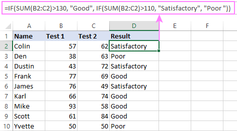
In some situations, your business logic may require including the SUM function in the logical test of IF. For example, to return different text labels depending on the sum of the values in B2 and C2, the formula is:
=IF(SUM(B2:C2)>130, "Good", IF(SUM(B2:C2)>110, "Satisfactory", "Poor"))
If the sum is greater than 130, the result is "good"; if greater than 110 – "satisfactory', if 110 or lower – "poor".
In a similar fashion, you can embed the AVERAGE function in the logical test of IF and return different labels based on the average score:
=IF(AVERAGE(B2:C2)>65, "Good", IF(AVERAGE(B2:C2)>55, "Satisfactory", "Poor"))
Assuming the total score is in column D, you can identify the highest and lowest values with the help of the MAX and MIN functions:
=IF(D2=MAX($D$2:$D$10), "Best result", "")
=IF(D2=MAX($D$2:$D$10), "Best result", "")
To have both labels in one column, nest the above functions one into another:
=IF(D2=MAX($D$2:$D$10), "Best result", IF(D2=MIN($D$2:$D$10), "Worst result", ""))

Likewise, you can use IF together with your custom functions. For example, you can combine it with GetCellColor or GetCellFontColor to return different results based on a cell color.
In addition, Excel provides a number of functions to calculate data based on conditions. For detailed formula examples, please check out the following tutorials:
Example 3. IF with ISNUMBER, ISTEXT and ISBLANK
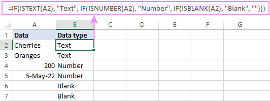
To identify text, numbers and blank cells, Microsoft Excel provides special functions such as ISTEXT, ISNUMBER and ISBLANK. By placing them in the logical tests of three nested IF statements, you can identify all different data types in one go:
=IF(ISTEXT(A2), "Text", IF(ISNUMBER(A2), "Number", IF(ISBLANK(A2), "Blank", "")))
Example 4. IF and CONCATENATE
To output the result of IF and some text into one cell, use the CONCATENATE or CONCAT (in Excel 2016 - 365) and IF functions together. For example:
=CONCATENATE("You performed ", IF(B1>100,"fantastic!", IF(B1>50, "well", "poor")))
=CONCAT("You performed ", IF(B1>100,"fantastic!", IF(B1>50, "well", "poor")))
Looking at the screenshot below, you'll hardly need any explanation of what the formula does:

IF ISERROR / ISNA formula in Excel
The modern versions of Excel have special functions to trap errors and replace them with another calculation or predefined value - IFERROR (in Excel 2007 and later) and IFNA (in Excel 2013 and later). In earlier Excel versions, you can use the IF ISERROR and IF ISNA combinations instead.
The difference is that IFERROR and ISERROR handle all possible Excel errors, including #VALUE!, #N/A, #NAME?, #REF!, #NUM!, #DIV/0!, and #NULL!. While IFNA and ISNA specialize solely in #N/A errors.
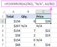
For example, to replace the "divide by zero" error (#DIV/0!) with your custom text, you can use the following formula:
=IF(ISERROR(A2/B2), "N/A", A2/B2)
And that's all I have to say about using the IF function in Excel. I thank you for reading and hope to see you on our blog next week!
Practice workbook for download
Excel IF multiple criteria - examples (.xlsx file)
 by
by
4506 comments
hi, i am trying to write a formula for the following:
80-100 , A
65-79, B
50-64, C
<50,F
but im not quite sure how to do that. can you please help me. thank you
Hi thank you for these blogs, I noticed above in this formula, =IF((C2+D2)>=60, "Good", IF((C2+D2)>=>40, "Satisfactory", "Poor ")) there is an extra >
If I could request your next lesson, it would be in arrays and tables within formulas. Thanks
Hi David,
Ah, good catch, many thanks! Fixed.
We already have a couple of tutorials on array formulas, hopefully they prove helpful:
Excel array formula examples for beginners and power users
Excel array formulas, functions and constants - examples and guidelines
Hi,
Can you help for following condition.,
Model Slab
Indica 1
Indica 2
MUV 1
MUV 2
using formula, if model indica, slab 1 means anws will be 100, if model indica, slab 2 means anws will be 200,if model MUV, slab 1 means anws will be 300, if model MUV, slab 2 means anws will be 400
how write the above formula.,
Hi
I am trying to do an Excel IF Array function.
I am trying to compare a country code, with that of a list of country codes, and let it return a specific value
Here is my formula =IF(A1='Eu Countries'!$D$2:$D$29,"EU","Non-EU")
It keeps returning False results, even though in my sample I can see countries and expect a True Value.
Please could you help.
Regards
Chrystian Michalowski
I am looking to only put 1 text if multiple values of a search is found in my search. Right now my formula will put multiple values in the output. The formula I am presently using is :
=IF(ISNUMBER(SEARCH("TEXT1",B2)),"EXEMPT","") & IF(ISNUMBER(SEARCH("TEXT2",B2)),"EXEMPT","") & IF(ISNUMBER(SEARCH("TEXT3",B2)),"EXEMPT","") & IF(ISNUMBER(SEARCH("TEXT4",C2)),"EXEMPT","")
If this matches 2 conditions it puts in EXEMPTEXEMPT
What I would like to find is if any of the criteria matches write exempt.
If (TEXT1 in B2) OR (TEXT2 in B2) OR (TEXT3 in B2) OR (TEXT4 in C2)then write EXEMPT otherwise leave blank
Hi,
Im trying to use the formula IF to do the following:
If in Cell P9 = PASS then Cell Q9 displays a value i have logged in cell P2 (which I have named the cell scpass) in same respect if P9 = FAIL then the value shown in Q9 displays a value I have logged in P3 (again I have named this cell SCFAIL)
I have used this formula =IF(P9="PASS","SCPASS","")&IF(P9="FAIL","SCFAIL","")
It works but rather than show the value logged in these cells it just displays the name I have put in the formula...
Please help!!
Adam,
On the formula you used when you break it down:
=IF(P9="PASS","SCPASS"," "") - When you type the word PASS on cell P9 then Excel goes to the next string which is the true statement and you have indicated to be true is the actual word "SCPASS". What you want to do is to reference the cells P2,Q2 in the formula for your true statement. If you change the words in cell P2 or Q2 then if would reflect in the formula what you typed on the cell.
Do this instead:
=IF(P9="PASS",P2,"")&IF(P9="FAIL",Q2,"")
I'm looking for a formula so I can make the text in one cell appear in another, within my IF statement.
Eg:
A B C
Anna 90 This is an excellent score, (Anna) should be very proud of herself
How can I tell excel to write the text in (e.g.) cell A1 into (e.g.) cell C1, while still using the IF statement for cell (e.g.) B1?
Katherine,
Below is I think what you were looking for. This is a simple one with cell A1= "A" and cell A2 would be Anna. The formula can be located in any cell. Would get intensive if you have multiple names and grades if this is what you are trying to accomplish.
=IF(A1="A",A2 &" " &B2 &" This is an excellent score, (" &A2 &" ) should be very proud of herself."," ")
=IF(Q4=1,"A",IF(Q4=2,"B",IF(Q4=3,"C",IF(Q4=4,"D",IF(Q4=5,"E",IF(Q4=6,"F",IF(Q4=7,"Provisional")))))))
Hi ive used the above formula to return a text response to a number result but its not working consistently. The number can be from 1-8 and there are corresponding text responses for each. What can i do?
Cheers
L
Lorraine,
Not sure what you are trying to accomplish but if cell Q4 is your input value and the formula that you have done is located on another cell. The formula works as long as Q4 is where you type your input numbers.
The number can only be from 1-7. If you type 8 or any other number the cell in your formula would indicate "FALSE" due to the "If statement" only has 7 conditions to check starting from 1 and end in 7.
=IF(Q43>=8,"Probationary",IF(Q43>6,"Provisional",IF(Q43>5,"F",IF(Q43>4,"E",IF(Q43>3,"D",IF(Q43>2,"C",IF(Q43>1,"B","A")))))))
Hi Pete, thanks for your response. I've changed the formula to be whats above which appeared to work but again its not consistent. I have 2 examples where the number in the target cell, in this case Q43, has been 6 and the response returned in the destination cell was "provisional" whilst other cells have shown the correct response of 'F". The numbers 1-8 are results of a median formula in the adjacent column.
Any further thoughts?
Hello again, ive looked at the entries again and there appears to be something in the array of numbers that may explain whats happening... (then again i might just have come across a coincidence!)
Examples are two median results of '5' but one is showing an 'E' response and the other an 'F'
The median of the number sets when written out are almost identical:
1st one: 4,4,5,5,5,6,6,6,7
2nd one: 4,4,5,5,5,6,6,7,7
both median numbers are 5 with a 5 and a 6 on either side.
I also considered using the mean value (which could work with these examples as there are no outliers) and when you look at the mean of these number sets the 1st is 4.2 (rounded to 4) and the latter 4.9 (rounded to 5). I need the median when i consider the purpose of this exercise and other examples - there are 87 rows of data) and in some examples the mean is not reflective.
Could the use of the median be the issue?
Lorraine,
Based on what you are testing to get the results.
Using the mean can give an erroneous result which may not be what you want when using your new "If" statements with the greater than test. Sometimes excel may show a number but the calculation may not reflect the result.
Median seam to work with your test to get the calculations and result that you would be expecting.
i have only one doubt which is:
i have in E1,drop down list,and i have in I1 the Qty, and J1 the price, and K1 the Net price,
what i want exactly to choose only 2 types from the drop down list.
which means
if x or Y in the drop down list, should the following:
I1*J1/2 and the same i want for Y, else i want I1*J1
Hi Svetlana Cheusheva,
=IF(E142000,E143500,E145000,E147500,"-$3.00","")
My formula as above, why my as above value never deduct inside the SUM total?
Any formula i missing out in above formula?
Hello May,
The syntax of this formula is wrong (or maybe it was broken by our blog engine when posting, sorry if it's the case). Anyway, you should never use any currency signs like $ in Excel formulas because it's only a visual representation of the underlying value. Also, surrounding a number in double quotes turns it into a text string, and as the result Excel cannot perform any calculations on it.
If you can explain what the formula is supposed to do, I will try to help you make it right.
what is the expected result of following formula?
=IF(2<3,IF(4<3,1+1,2+2),3+3)
It's 4.
I need to know what is the right way to have both AND OR in one statement.
A and B have 3 status C, N, or O;
If (A=C or A=N) AND (B=C or B=N), output should be C, otherwise is O
Thank you.
Hi Frieda,
Here you go:
=IF(AND(OR(A1=C1, A1=N1), OR(B1=C1, B1=N1)), C1, 0)
I am trying to create two IF statements.
1) If the due date is equal to/less than 30 days the text should read "In Progress"
2) If the due date is greater than 30 days the cell should be Bank ""
I can't figure out why this formula isn't working:
=IF(e2="AB", (F2="Cash", J2, (J2*40%)), IF(E2="LSI", (F2="Cash", J2, (J2*60%)))
Christie,
This is a logical function where the "IF" and "AND" operators need to be involved. Is this what you were looking for on the formula to do.Try this revision to your formula above.
You can also use a drop down on cell E2 instead of typing the two words.
=IF(AND(E2="AB",F2="Cash"),J2*0.4,IF(AND(E2="LSI",F2="Cash"),J2*0.6))
Hi im trying to use a drop down list by in cooperating it with a nested if statement. the drop down list is on B8 therefore I want to derive the diff values from the list. How do I write that formula
Hi Svetlana,
Pls what formula do I use to calculate, lets say, the number of "A"s in a group of grades?
example,
Final Grade
74.1 A
52.2 C
69.6 B
32 F
70.2 A
45.6 D
47.1 D
53 C
41.4 D
59.3 C
30 F
45 D
63.7 B
73.2 A
71.2 A
GRADE NUMBER
A ??
B ??
C ??
D ??
F ??
Pls help. Thanks
Hi Usman,
You can use the COUNTIF function for this. For example:
=COUNTIF(B:B, "A")
Where B is the column containing grades.
Dear Svetlana Cheusheva i need help for following conditional formula
Suppose Buyer Name is "K-Mart, H&M" and Fabrics types is "General,Ordinary and Special) length range in (+-5) and width range in (+-7) its will be pass, if not its will be fail.
When change the value of Length and width then result will be changed.
If you help me i will be grateful to you.
I have worksheet that lists int exp and payment for multiple leases. I'm manually opening each amtz schedule and inputing these into each column,each month. I would like to write a formula that will say when the lease number in column A matches a lease from one the amtz schedules, and when the date matches, lookup the int exp and return in column O.
=IF(B2>90,"A",IF(B2>80,"B",IF(B2>70,"C",IF(B2>60,"D",IF(B2="absent","F","F")))))
i want to excel display F for absent also.
I am trying to write a nested formula. The first vlookup works, however the second and third vlookups are not working. Can anyone tell me what i am doing wrong please?
=IFERROR(IF(AB2="Other",VLOOKUP(M2,'price list'!A$2:$N$1247,13,FALSE),IF(AB2="Sysco",VLOOKUP(L2,'Sysco US Foods Pricelist'!$A$5:$J$214,5,FALSE),IF(AB2="USF",VLOOKUP(L2,'Sysco US Foods Pricelist'!$A$5:$J$214,10,FALSE),0))),0)
Hi,
i want to write a formula in C1
column A1 date is less or equal to today date then = Yes
column B1 date is less or equal to today date then= No
if both are less or equal to today date then= Both.
please help me out.
i tried if & And but not successes.
Girish
Hi,
I'm trying to create an If function that would evaluate a score, then based on that score value predict a future test date based off of the date the first test was taken. Here are two examples:
1.) TESTED: 1/1/2015 SCORE:>70 NEXT TEST:12 months from first date(1/1/2016) 2.) TESTED: 1/1/2015 SCORE:<70 NEXT TEST:6 months from first date(7/1/2016) Do you have any idea how to format this correctly? Every time I try, I end up with either an error, or the result of my text. Thanks!
I am trying to create above formula to find the efforts based upon the inputs from respective columns as referred, but with 1-1 its returning right when i am trying to add multiple conditions its not working for which need help.
Below Query1 for one condition but the second query tried to build for another condition its returing Medium value everytime.
Columns: Technology || No. Of Interfaces || Interface Type || Phases || Complexity || Total Efforts
Query1: =IF(AND(A3="SOA", C3="New", D3="Requirement", E3="Simple", OR(A3="SOA", C3="Enhancement", D3="Requirement", E3="Simple")), B3*'Efforts Summary'!C3, B3*0.6*'Efforts Summary'!C3)
Query2:=IF(IF(AND(A3="SOA", C3="New", D3="Requirement", E3="Simple", OR(A3="SOA", C3="Enhancement", D3="Requirement", E3="Simple")), B3*'Efforts Summary'!C3, B3*0.6*'Efforts Summary'!C3), IF(AND(A3="SOA", C3="New", D3="Requirement", E3="Medium", OR(A3="SOA", C3="Enhancement", D3="Requirement", E3="Medium")), B3*'Efforts Summary'!D3, B3*0.65*'Efforts Summary'!D3))
I need to add similary for design, build, test along with complex category overll.
Appreciate if anybody can provide some help here.
Hi Savetlana,
when I input 17 or 20 digits in Cell F8 the result should be "Pass" otherwise "Fail"
also note that I am checking the length of digits in the cell.
below condition is not showing positive result.
=IF(OR(LEN(F8)=17, LEN(F8)=20), "Pass", "Fail")
Regards,
Khalid
Please use:
=IF(AND(LEN(F8)>=17, LEN(F8)<=20), "Pass", "Fail")
Please give a formula to get answer for the following:
TDS (Tax deducted from source) 10% for employees below Gross pay Rs.15000 and for other employees 20% ?
Hello,
I have a question, in my worksheet i have 2 cell where i have to input value "O13 & Y13", now i want an alert to be flashed if a value is entered in O13 and not in Y13 & vice-versa, how can i do it.
awaiting your earlist reply.
Regards
Karan
I am using below
=IF(OR(AND(LEN(TRIM(F8 = 17)), AND(LEN(TRIM(F8 = 20))))), "Pass", "Fail")
Hello Khalid,
From your formula, it's difficult to understand what result you are trying to achieve. I have the following suggestions:
Show "Pass" if cell F8 contains 17 or 20 characters, "Fail" otherwise:
=IF(OR(LEN(F8)=17, LEN(F8)=20), "Pass", "Fail")
Show "Pass" if the value in cell F8 is either 17 or 20, "Fail" otherwise:
=IF(OR(F8=17, F8=20), "Pass", "Fail")
If you are looking for something different, please clarify.
Hi Team,
please find below condition is not working. I am trying to if value is 17 and 20 so result should "Pass" otherwise "fail" but value is showing every time "Pass" with wrong input and right value. kindly check and advise on urgent basis.
=IF(OR(AND(LEN(TRIM(F8 = 17)), AND(LEN(TRIM(F8 = 20))))), "Fail", "Pass")
Regards,
Khalid
Hi there,
I'm trying to calculate how many months a participant stays in a job, based on a start date in one column and in the next column, each cell is either blank (if they're still employed) or has an end date if they lost their job. I'm trying to figure out a formula that will calculate the months between column J (start date) and column K (end date, if there is one)... so that the number of months will show up in another separate column. If there is a blank, I want the number of months to be calculated between the start date and today's date... I tried to combine formulas and came up with what I copy/pasted below, but it's not working... Is this possible and can you help me figure out a formula that will do what I want?
Formula that isn't working:
=IF(ISDATE(K2), (YEAR(K2)-YEAR(J2))*12+MONTH(K2)-MONTH(J2), IF(ISBLANK(B1), (DAY(NOW())>=DAY(J2),0,-1)+(YEAR(NOW())-YEAR(J2)) *12+MONTH(NOW())-MONTH(J2), "")))
Hi Svetlana,
I'm trying to work out commission structures in excel, for example if the fee is less than 10k, then the commission is 10%, if fee is more than 10k but less than or equal to 20k, then 10% of the first 10k + 20% of anythingthing between 10-20k, and then 10% of 0-10k, 20% of 10-20k, 30% of 20-30k etc and 40% of everything above 30k.
Please help!
Kind Regards
Tom
i am trying to output a letter code base on ranges for example if a cell has numbers from:
-1 to -26 should output text "A"
-27 to -54 "B"
55 TO 25 "C"
24 TO 6 "D'
5 TO 1 "E"
for example if a cell has -23 output would be A
i tried some of the above but often i get EBC various letters together
Hello Joe,
Try the following formula:
=IF(AND(A1>=25, A1<=55), "C", IF(A1>=6, "D", IF(A1>=1, "E", IF(A1>=-26, "A", IF(A1>=-54, "B", "")))))
Hi ,
I Good tools however i need to add more conditions in the same formula but i was not applied
Mistake Severity One Cases Two Cases Three Cases Four Cases
Critical 10% 20% 30% 40%
Hard 7% 14% 21% 28%
Normal 3% 6% 9% 12%
Repeated 3% 6% 9% 12%
Human error 1% 2% 3% 4%
I'm having trouble building the proper if function for what I need and would appreciate any help!
I'm in need of a formula which adds different amounts based on a SUM amount. The SUM is cell D15.
Example IF(D15>=0.55, D15+.25)
My problem is that I need this for several different number ranges, and all in the same cell.
If D15=25or higher, D15+3
If D15=15-24.99, D15+1.75
If D15=10-14.99, D15+1.5
If D15=7-9.99, D15+1
If D15=5-6.99, D15+.75
If D15=3-4.99, D15+.55
If D15=0.56-2.99, D15+.5
If D15=0.01-0.55, D15+.25
If D15=0, 0
I hope this makes sense. Mostly it is difficult for me because there are so many variables. Any help would be appreciated!
Hi,
could you please help me with the below:
=IF(VLOOKUP(N9;zonespecific.loc.!R:S;2;0)<200;"Replenish";"OK")&IFERROR(VLOOKUP(N14;zonespecific.loc.!R:S;2;0);"Not in stock")
I am trying to nest a iferror function into the if function to highlight with my specified criteria the cell when the if function is not applicable but I am not able to get it right.
Thank you in advance
Hi
I'm trying to create a formula to total a cell based on two conditions
Column D is titled Activity: Running, Cycling (Condition 1)
Column K is titled Distance: 5, 10
Column S is titled Company: Paul, John (Condition 2)
I can calculate the total amount of running and cycling by using this formula =SUMIF(D3:D57,"Running",I3:I57)
What I want to do is expand this formula to calculate the amount of running with John or Paul only based on Column S.
Can you help?
Thanks Paul
Hi Paul,
To sum cells with several conditions, you need to use the SUMIFS function rather than SUMIF. For example:
=SUMIFS(I3:I57, D3:D57,"Running", C3:C57,"Paul")
That worked perfectly.. I just copied in your formula :-)
Thank you so very much you are exceptional.
Paul
please excel format how could multiply and subtract in the excel formats.
goodevening :D can you help on what is the formula of this?
A Route is Classified as LONG Haul if the destination is further than 1000 miles From UK and SHORT Haul if less. (Use Absolute Reference)
I am working on the excel sheet in which i have to put the following conditions like
if gpa is in the range of 3.81- 4.00 then assign the marks 20
if the gpa in the range of 3.61- 3.80 then assign the marks 10 and so on for the other gpa what is the solution to this kindly any one can help me
Thanks
Hi Nayab,
You can write a nested If formula similar to this:
=IF(A1>3.8, 20, IF(A1>3.6, 10, IF(...)))
Hello
I would like to know how to use nested loop functions with logical operator AND, using data from columns in different sheets.
Like for instance, if there has to be condition placed such that if Column D in Sheet1 AND Column D in Sheet2 AND Column D in Sheet3 AND Column D in Sheet4 are true, the result is RANK1 in Column B in Sheet5?
How to go about it? I hope I have made myself clear.
Hi
am trying to create a formula in excel 2010
=IF(C5=10918,(IF(AY5*0.02<10,10,IF(AY5<0,0,AY5*0.02))),IF(C5=14449,IF(D5=0,0,(D5-S5)/1.145)),IF(C5=32466,IF(D5*0.02<10,10,D5*0.02))
but it is showing too many arguments for this functions, am planing to use more thn 50 ifs here, is it even possible??
Hi,
I am trying to create a formula that will insert one of four colored symbols. For example if cell value is >= 96% insert solid blue circle, if btwn 93% and 96% insert solid green circle. Etc.
Thanks for your help!
hi
have prep this string
=CONCATENATE(IF(C2=10918,(IF(AY2*0.02<10,10,IF(AY2<0,0,AY2*0.02))),IF(C2=14449,(D2-S2/1.145))),IF(C2=17178,(IF(D2=0,0,IF(D2<230,4,D2*2/100)))),IF(C2=32466,IF(D2=0,0,IF(D20.4,VLOOKUP(C2,'Merchant ID'!A:E,3,0))*D2)
but am getting
FALSEFALSE100
am confused what am doing wrong, help me out?
=IF(D8>D34,5,IF(D8=D34,4,IF(AND(D8=(D34-2)),2,IF(AND(D8=(D34-3)),1,IF(D8<=0%,0)))))
Id like to correct my previous, This is my actual formula
I've been trying to create formula on this:
Higher than inflation rate, the score is 5
Within inflation rate, score is 4
2 points below inflation rate, score is 2
3 points or more below the inflation rate, score is 1
At 0% or negative, score is 0.
So I entered the following formula, where D8 contains the score, and D34 is where I entered the inflation rate. But it doesn't work.
=IF(D8>D34,5,IF(D8=D34,4,IF(AND(D8=(D34-2)),2,IF(AND(D8=(D34-3)),1,IF(D8<=0%,0)))))
I'm trying to create 5 new character variables from a set of 5 existing variables (test scores - math, lang, phys, soci, comp). The goal is to create a new variable for each score, based on a set of cutpoints of the test score. The comp variable -- a summary or overall variable -- can be either numeric or character. The two character options for comp are "Incomplete" and "Other", and are valid values when there is a missing score for any one of the the other 4 variables. Let's say that the first row of 5 original variables are in cells A2, B2, C2, D2, and E2. If there are numeric values in each of those cells, the formula would be written: =IF(A2>=270|"Demonstrating"|IF(A2<258|"Emerging"|"Approaching")). Where I'm stuck is in writing the formula for when there is a blank value in one of the 4 test score fields (A2, for example). Can you help?
There are 1000 values in one column (C). I need to populate the value '1', if the value in column (C) is equal to 'A','B','C','D' or 'E'. Else, I need it to populate zero. Basically, my simple formula of =if(C1="A",1,0) needs to be extended to A or B or C or D or E - all in one cell formula itself.
Hi Gurgaa,
Simply embed the OR function in your formula, like this:
=if(OR(C1="A", C1="B", C1="C", C1="D"), 1, 0)
Hello dear Svetlana,
If add one more part that is, if cell5 (total) be between 50 and 59 grade C, between 60 and 79 B, between 80 and 100 grade A (for level1,level2 and level3). if cell5(total be between 60 and 65 grade C, between 65 and 79 grade B, between 80 and 100 grade A.
your kindness will be highly appreciated.
Hi Gul Mohammad,
You can use the following nested If functions to display grades in a separate cell:
=IF(AND(OR(A4="level1", A4="level2", A4="level3", A4="level4", A4="level5"), A5>=80), "A", IF(AND(OR(A4="level1", A4="level2", A4="level3"), A5>=60), "B", IF(AND(OR(A4="level1", A4="level2", A4="level3"), A5>=50), "C", IF(AND(OR(A4="level4", A4="level5"), A5>=65), "B", IF(AND(OR(A4="level4", A4="level5"), A5>=60), "C", "")))))
Hi Svetlana:
I think you missed one and that is,you have not specified the Grade A for level four and level five. Now how do i continue?
should I just add like the others?
Hi Gul Mohammad,
Because Grade A is identical (between 80 and 100) for all the levels, I added 5 levels in the first logical test to make the formula a bit more compact.
If you don't mind one more problem that I faced with, and really disturbs me is that how to solve this of course it is in connection with previous.
if cell4= level1,level2,level3 and at the same time total(cell5) be greater than 50 pass and otherwise fail and at the same time if total be between 50 and 59 that grade must be C, if between 60 and 79 grade must be B and if between 80 and 100 grade must be A.
But if cell4= level4,level5 and at the same time cell5(total) be greater than 60, rusult be pass and otherwise fail and at the same time if cell5(total) be between 60 and 65 grade C, between 65 and 79 grade B, between 80 and 100 grade A.
Thank you so much once again.
Thank you too much for helping us. I will appreciate if you could help me with this function.Suppose if cell4= level1,level2,level3 and at the same time cell5(total score) be greater than 50,the student is pass otherwise fail.
And again if cell4= level4,level5 and at the same time cell5(total score) be greater than 60, the student is pass otherwise fail.
It will be your kindness if you could help to handle it.
Hello Gul Mohammad,
Try the following formula:
=IF(OR(AND(OR(A4="level1", A4="level2", A4="level3"), A5>50), AND(OR(A4="level4", A4="level5"), A5>60)), "pass", "fail")
Thank you so much dear Svetlana Cheusheva.
It really helps me.
I appreciate your helping and also your talent.
best wishes
Is there any formula for the condition where have to use "OR" more than twice.
ex:
A B C D Y=YES
Y N N Y N=NO
I want a condition : =if(A OR B OR C OR D ="Y","AGREE","NA")
i want to use "or" more than twice. Is it possible?
Hello Naveen,
Of course, it's possible. Like in any other Excel function, you can include up to 255 arguments in an OR statement as long as the total length of your formula does not exceed 8,192 characters :)
=IF(OR(A1="Y", B1="Y", C1="Y", D1="Y"),"AGREE","NA")
Hi Svetlana,
For Naveen's query we could also use this formula
=IF(B1="A","Y",IF(B1="B","Y",IF(B1="C","Y",IF(B1="D","Y",IF(B1="Y","N",IF(B1="N","N"""))))))
Substituting any other text for "Y" or "N" within the brackets.
But don't you think that a Table with the two columns - one with the condition and other with the output/result, will help this problem with a Vlookup formula. The table can be expanded without having to expand the formula or make it more complex.
I have been using this method with excellent results and as an Excel professional I would be glad to know your views.
Regards,
Ramki