The tutorial shows how to create multiple IF statements in Excel with AND as well as OR logic. Also, you will learn how to use IF together with other Excel functions.
In the first part of our Excel IF tutorial, we looked at how to construct a simple IF statement with one condition for text, numbers, dates, blanks and non-blanks. For powerful data analysis, however, you may often need to evaluate multiple conditions at a time. The below formula examples will show you the most effective ways to do this.
How to use IF function with multiple conditions
In essence, there are two types of the IF formula with multiple criteria based on the AND / OR logic. Consequently, in the logical test of your IF formula, you should use one of these functions:
- AND function - returns TRUE if all the conditions are met; FALSE otherwise.
- OR function - returns TRUE if any single condition is met; FALSE otherwise.
To better illustrate the point, let's investigate some real-life formulas examples.
Excel IF statement with multiple conditions (AND logic)
The generic formula of Excel IF with two or more conditions is this:
Translated into a human language, the formula says: If condition 1 is true AND condition 2 is true, return value_if_true; else return value_if_false.
Suppose you have a table listing the scores of two tests in columns B and C. To pass the final exam, a student must have both scores greater than 50.
For the logical test, you use the following AND statement: AND(B2>50, C2>50)
If both conditions are true, the formula will return "Pass"; if any condition is false - "Fail".
=IF(AND(B2>50, B2>50), "Pass", "Fail")
Easy, isn't it? The screenshot below proves that our Excel IF /AND formula works right:

In a similar manner, you can use the Excel IF function with multiple text conditions.
For instance, to output "Good" if both B2 and C2 are greater than 50, "Bad" otherwise, the formula is:
=IF(AND(B2="pass", C2="pass"), "Good!", "Bad")
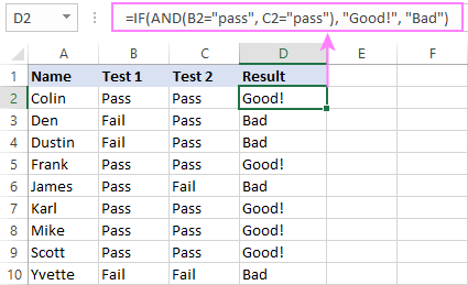
Important note! The AND function checks all the conditions, even if the already tested one(s) evaluated to FALSE. Such behavior is a bit unusual since in most of programming languages, subsequent conditions are not tested if any of the previous tests has returned FALSE.
In practice, a seemingly correct IF statement may result in an error because of this specificity. For example, the below formula would return #DIV/0! ("divide by zero" error) if cell A2 is equal to 0:
=IF(AND(A2<>0, (1/A2)>0.5),"Good", "Bad")
The avoid this, you should use a nested IF function:
=IF(A2<>0, IF((1/A2)>0.5, "Good", "Bad"), "Bad")
For more information, please see IF AND formula in Excel.
Excel IF function with multiple conditions (OR logic)
To do one thing if any condition is met, otherwise do something else, use this combination of the IF and OR functions:
The difference from the IF / AND formula discussed above is that Excel returns TRUE if any of the specified conditions is true.
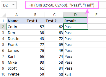
So, if in the previous formula, we use OR instead of AND:
=IF(OR(B2>50, B2>50), "Pass", "Fail")
Then anyone who has more than 50 points in either exam will get "Pass" in column D. With such conditions, our students have a better chance to pass the final exam (Yvette being particularly unlucky failing by just 1 point :)
Tip. In case you are creating a multiple IF statement with text and testing a value in one cell with the OR logic (i.e. a cell can be "this" or "that"), then you can build a more compact formula using an array constant.
For example, to mark a sale as "closed" if cell B2 is either "delivered" or "paid", the formula is:
=IF(OR(B2={"delivered", "paid"}), "Closed", "")
More formula examples can be found in Excel IF OR function.
IF with multiple AND & OR statements
If your task requires evaluating several sets of multiple conditions, you will have to utilize both AND & OR functions at a time.
In our sample table, suppose you have the following criteria for checking the exam results:
- Condition 1: exam1>50 and exam2>50
- Condition 2: exam1>40 and exam2>60
If either of the conditions is met, the final exam is deemed passed.
At first sight, the formula seems a little tricky, but in fact it is not! You just express each of the above conditions as an AND statement and nest them in the OR function (since it's not necessary to meet both conditions, either will suffice):
OR(AND(B2>50, C2>50), AND(B2>40, C2>60)
Then, use the OR function for the logical test of IF and supply the desired value_if_true and value_if_false values. As the result, you get the following IF formula with multiple AND / OR conditions:
=IF(OR(AND(B2>50, C2>50), AND(B2>40, C2>60), "Pass", "Fail")
The screenshot below indicates that we've done the formula right:
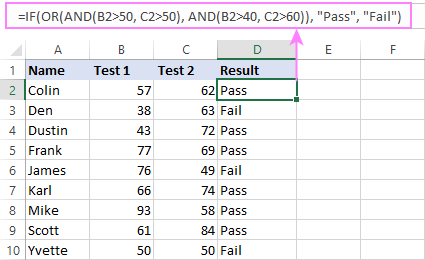
Naturally, you are not limited to using only two AND/OR functions in your IF formulas. You can use as many of them as your business logic requires, provided that:
- In Excel 2007 and higher, you have no more than 255 arguments, and the total length of the IF formula does not exceed 8,192 characters.
- In Excel 2003 and lower, there are no more than 30 arguments, and the total length of your IF formula does not exceed 1,024 characters.
Nested IF statement to check multiple logical tests
If you want to evaluate multiple logical tests within a single formula, then you can nest several functions one into another. Such functions are called nested IF functions. They prove particularly useful when you wish to return different values depending on the logical tests' results.
Here's a typical example: suppose you want to qualify the students' achievements as "Good", "Satisfactory" and "Poor" based on the following scores:
- Good: 60 or more (>=60)
- Satisfactory: between 40 and 60 (>40 and <60)
- Poor: 40 or less (<=40)
Before writing a formula, consider the order of functions you are going to nest. Excel will evaluate the logical tests in the order they appear in the formula. Once a condition evaluates to TRUE, the subsequent conditions are not tested, meaning the formula stops after the first TRUE result.
In our case, the functions are arranged from largest to smallest:
=IF(B2>=60, "Good", IF(B2>40, "Satisfactory", "Poor"))
Naturally, you can nest more functions if needed (up to 64 in modern versions).

For more information, please see How to use multiple nested IF statements in Excel.
Excel IF array formula with multiple conditions
Another way to get an Excel IF to test multiple conditions is by using an array formula.
To evaluate conditions with the AND logic, use the asterisk:
To test conditions with the OR logic, use the plus sign:
To complete an array formula correctly, press the Ctrl + Shift + Enter keys together. In Excel 365 and Excel 2021, this also works as a regular formula due to support for dynamic arrays.
For example, to get "Pass" if both B2 and C2 are greater than 50, the formula is:
=IF((B2>50) * (C2>50), "Pass", "Fail")

In my Excel 365, a normal formula works just fine (as you can see in the screenshots above). In Excel 2019 and lower, remember to make it an array formula by using the Ctrl + Shift + Enter shortcut.
To evaluate multiple conditions with the OR logic, the formula is:
=IF((B2>50) + (C2>50), "Pass", "Fail")
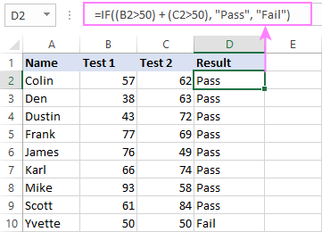
Using IF together with other functions
This section explains how to use IF in combination with other Excel functions and what benefits this gives to you.
Example 1. If #N/A error in VLOOKUP
When VLOOKUP or other lookup function cannot find something, it returns a #N/A error. To make your tables look nicer, you can return zero, blank, or specific text if #N/A. For this, use this generic formula:
For example:
If #N/A return 0:
If the lookup value in E1 is not found, the formula returns zero.
=IF(ISNA(VLOOKUP(E1, A2:B10, 2,FALSE )), 0, VLOOKUP(E1, A2:B10, 2, FALSE))
If #N/A return blank:
If the lookup value is not found, the formula returns nothing (an empty string).
=IF(ISNA(VLOOKUP(E1, A2:B10, 2,FALSE )), "", VLOOKUP(E1, A2:B10, 2, FALSE))
If #N/A return certain text:
If the lookup value is not found, the formula returns specific text.
=IF(ISNA(VLOOKUP(E1, A2:B10, 2,FALSE )), "Not found", VLOOKUP(E1, A2:B10, 2, FALSE))

For more formula examples, please see VLOOKUP with IF statement in Excel.
Example 2. IF with SUM, AVERAGE, MIN and MAX functions
To sum cell values based on certain criteria, Excel provides the SUMIF and SUMIFS functions.
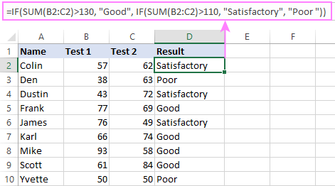
In some situations, your business logic may require including the SUM function in the logical test of IF. For example, to return different text labels depending on the sum of the values in B2 and C2, the formula is:
=IF(SUM(B2:C2)>130, "Good", IF(SUM(B2:C2)>110, "Satisfactory", "Poor"))
If the sum is greater than 130, the result is "good"; if greater than 110 – "satisfactory', if 110 or lower – "poor".
In a similar fashion, you can embed the AVERAGE function in the logical test of IF and return different labels based on the average score:
=IF(AVERAGE(B2:C2)>65, "Good", IF(AVERAGE(B2:C2)>55, "Satisfactory", "Poor"))
Assuming the total score is in column D, you can identify the highest and lowest values with the help of the MAX and MIN functions:
=IF(D2=MAX($D$2:$D$10), "Best result", "")
=IF(D2=MAX($D$2:$D$10), "Best result", "")
To have both labels in one column, nest the above functions one into another:
=IF(D2=MAX($D$2:$D$10), "Best result", IF(D2=MIN($D$2:$D$10), "Worst result", ""))

Likewise, you can use IF together with your custom functions. For example, you can combine it with GetCellColor or GetCellFontColor to return different results based on a cell color.
In addition, Excel provides a number of functions to calculate data based on conditions. For detailed formula examples, please check out the following tutorials:
Example 3. IF with ISNUMBER, ISTEXT and ISBLANK
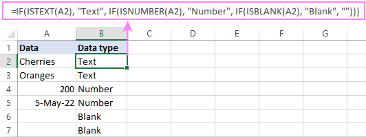
To identify text, numbers and blank cells, Microsoft Excel provides special functions such as ISTEXT, ISNUMBER and ISBLANK. By placing them in the logical tests of three nested IF statements, you can identify all different data types in one go:
=IF(ISTEXT(A2), "Text", IF(ISNUMBER(A2), "Number", IF(ISBLANK(A2), "Blank", "")))
Example 4. IF and CONCATENATE
To output the result of IF and some text into one cell, use the CONCATENATE or CONCAT (in Excel 2016 - 365) and IF functions together. For example:
=CONCATENATE("You performed ", IF(B1>100,"fantastic!", IF(B1>50, "well", "poor")))
=CONCAT("You performed ", IF(B1>100,"fantastic!", IF(B1>50, "well", "poor")))
Looking at the screenshot below, you'll hardly need any explanation of what the formula does:

IF ISERROR / ISNA formula in Excel
The modern versions of Excel have special functions to trap errors and replace them with another calculation or predefined value - IFERROR (in Excel 2007 and later) and IFNA (in Excel 2013 and later). In earlier Excel versions, you can use the IF ISERROR and IF ISNA combinations instead.
The difference is that IFERROR and ISERROR handle all possible Excel errors, including #VALUE!, #N/A, #NAME?, #REF!, #NUM!, #DIV/0!, and #NULL!. While IFNA and ISNA specialize solely in #N/A errors.
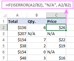
For example, to replace the "divide by zero" error (#DIV/0!) with your custom text, you can use the following formula:
=IF(ISERROR(A2/B2), "N/A", A2/B2)
And that's all I have to say about using the IF function in Excel. I thank you for reading and hope to see you on our blog next week!
Practice workbook for download
Excel IF multiple criteria - examples (.xlsx file)
 by
by
4506 comments
Hi Svetlana,
Need your help
I want a formula for these conditions
If the labour take leave more than 5 days the value should be "no. of leave days".
If the labour take leave less than 5 days the value should be "0".
ex.
8 days leave means ans should be "8".
4 days leave means ans should be "0".
Hi Saravana,
You can use a formula similar to this:
=IF(A1>=5, A1, 0)
where A1 is the cell containing the number of leave days.
Hi Svetlana,
Need your help
i was trying the formula unfortunately something wrong can you pls help
Name Start time log in time
12:30 12:40 late login
12:30 12:30 on time
12:30
=IF(C2-B2>0,"late login","on time")
when the third column is nil i have put the fourmula
=IF(C4-B4>0,"late login","on time",if(c4="","leave")).
Thanks and regards
Giriraj
Hi Giriraj,
Try the following syntax:
=IF(C2="","leave", IF(C2-B2>0,"late login","on time"))
Hi,
I need a formula to calculate the below conditions.
if 800 is 160% of 500, first 100% should be calculated in .1% and next 50% should be calculated in .2% and remaining 10% should be calculated in .25%.
Please help
I'm trying to merge multiple workbooks/sheets into 1 master. I have a template that someone made (who know who) that works but only to a certain row and not through out the workbook so when I copy and paste or when I consolidate the formula/condition doesn't transfer so I wanted to create one from scratch.
Here's the criteria:
The row will highlight yellow if at least one of the grades in either column E or F is less than 73.
The row will highlight red if both grades are less than 73.
Help please! I've Googled, YouTube, and even taken a a short course and nothing.
I have a tool size range and I'd like to determine if a given measurement falls within the range.
Column A is the RANGE (.7"-1.4")
Column C is a TOLERANCE such as (+/- .0001)
Column D is a target such as .75
Column E is the ACTUAL READING such as .1200
What would the formula be to determine if the value of Column E (ACTUAL READING) falls into the (RANGE) while taking the TOLERANCE into consideration? In this example .1200 does NOT fall within the range listed in Column A, but .80 DOES fall within the range.
Please help. Your answers look beautifully simple, but I'm not sure how to use them to solve my particular situation.
Thanks. so much!
Hi,
Can you help figure out what formula i'm going to use? i want to get the sum of the whole column with the same equivalent in other column. for example a1 to A10 has different value let say 2,3,4,5,6 and in B1 to B10 has its equivalent value like 100,123,121,333 etc. i want to get the sum of row with 2 value in B column and its total sum.
Hello Manny,
If my understanding is correct, you need to sum only those cells in column B, that have 2 in the same row in column A. If so, you can use the following SUMIF formula:
=SUMIF(A1:A10, 2, B1:B10)
Hi
Value in cell A3 is 10
I want to check this value tn 4 Different Criteria
1)Less than 20
2)Greater than 20 but less than 50
3)Greater than 50 but less than 80
4)greater than 80
Please help
Regards
Venkat
Hello!
I want to only bring back a value when column A shows "Project". I want to multiply 2 different columns together but the tricky part is that sometimes those fields are blank and it's returning a #Value! error which I would like to remove and show as a blank field.
Column A: "Project" Verbiage needed
Column B: Value 1 for multiplication (can be blank sometimes)
Column C: Value 2 for multiplication (can be blank sometimes)
If Column A = "Project", multiply column B x column C and if it returns a #Value error (from at least 1 field being blank), return an empty cell.
Thoughts? Thank you in advance!
Hello,
I am having trouble displaying multiple matches from nested IF statements.
As an example:
I have a meal planner with QUICK, CASUAL, EXTRAVAGANT. QUICK = =15 but 30.
Now say meal 1 takes 13-18 minutes, which puts it in Quick and Casual, but the validation stops after it meets the <15 logic, how can I get it to check the rest of the specifications to check the Casual block also?
Thanks for any help.
Sam
Something didn't post right.
Quick: first IF is less than or equal to 15, "QUICK" next IF equal or greater than 15 but less than equal to 30, "CASUAL", third IF equal to or greater than 30 "EXTRAVAGANT". The rest is correct as I put in a meal that takes 13-18 minutes, how to I have the formula block identify it as a Quick Casual Meal.
Thanks
Hi Sam,
You can use the following nested If functions:
=IF(A1>=30, "EXTRAVAGANT", IF(A1>=15, "CASUAL", "QUICK"))
Hi,
I need help combining 3 individual IF formulas into one. All work correctly as individual formulas but I can't figure out how to combine the 3 formulas into one. The individual formulas are as follows:
=IF(OR(ISNUMBER(SEARCH("TAMPA BAY*",C2)),ISNUMBER(SEARCH("TAMPA TRIBUNE*",C2)),ISNUMBER(SEARCH("TAMPA BAY NEWS*",C2)),ISNUMBER(SEARCH("LEDGER*",C2)),ISNUMBER(SEARCH("NEIGHBORHOOD*",C2)),ISNUMBER(SEARCH("OBSERVER*",C2))),"PN","NO")
=IF(OR(ISNUMBER(SEARCH("out*",C3)),ISNUMBER(SEARCH("CLEAR*", C3)),ISNUMBER(SEARCH("LAMAR*",C3))),"O","NO")
=IF(OR(ISNUMBER(SEARCH("Bright*",C4)),ISNUMBER(SEARCH("Com*", C4)),ISNUMBER(SEARCH("Via*",C4))),"C","NO")
Thanks for the help!
Mary
I have written this syntax:
=IF($V$5100%,C$23=8/1/16,IF(AND(C$23>100%,C$23<=115%),$Q$5*1.75,0))))
Why FALSE came up?
Hope you could help.
AM
let me make a bit more clear
I am a FOREX Currency Trader. I record all of my trades in a Trading Journal (excel file). I would like calculate the What is the Maximum Consecutive Winning or Loosing streak in number (don't want to add them together).
If we have over 1000 rows & there are positive & negative values in one column. I want a formula to take out the maximum consecutive values (either positive or negative). I tried a lot but couldn't workout. Please help.
Mark Sheet
StudentName Tamil English Hindi Maths
Arun 22 34 44 55
Vinoth 45 56 76 43
David 98 34 22 96
Vasanth 35 87 45 69
Andrew 78 89 98 74
Result
Student name-
Subject name-
Subject Mark-
Note:
1. Should Not use Vlooup
2. If Student name and subject name change in Result , automatically subject score should display.
3. The changes should done based on Mark Sheet given at above.
Good day I need to write an if formula on tax brackets.
If a person earns between 100 and 500 for example the tax will be X amount minus rebate of X amount. And if a person earns between 600 and 1000 the ta X will be a amount and the amount above X amount multiply with x% + a minus X amount rebate
a b c d
1 1 0 1
1 0 1 1
1 1 1 1
0 1 0 0
0 0 1 0
0 0 0 0
a, b and c are my conditions and d is my result so can I get the excel formula to get result for all six conditions.
I seem to be going around in circles, I have two fields, one contains First Names and the other Surnames. Most surnames are single names but some are two names hyphenated and some are two names with a space between them.
The end result I am looking for is for single surnames it will result in first character or first name followed by surname, no spaces.
Both hyphenated and spaced dual surnames will be first character of firstname, followed by first character of first surname followed by last surname. So somebody with a name of Peter Barkley Smith for instance will result in pbsmith.
I need help!! I am using the following formula:
=SUMIFS('OE761-2'!C:C,'OE761-2'!B:B,"SGIANNA",'OE761-2'!E:E,"="&J33)
Basically, I am summing the total in C:C if B:B has the name SGIANNA and the date in E:E is the same as the date in J33. It works just fine, but if the date in J33 is not found in E:E, I want to leave the cell blank. Any guidance would be much appreciated!
Hi..............
my question is???
My Product Name - Samsung-E1200 just time price - 1120/-
and then price drop it this product - Samsung-E1200 - 1175/-
so sir howes condition apply i m not understand????
so sir please suggest me............. and question is ????
01-feb to 14-feb price 1120/-
then 15-feb to 29-feb- price change 1175/-
so suggest me???????
Can anyone help me with this. I need an excel formula for the following. If there are 4 price ranges depending on volume sold, then what is the total revenue for a given volume sold?
For example
<10,000, price is 4
10,000 - 20,000, price is 3
20,000 - 30,000, price is 2
More than 30,000, price is 1
The formula should calculate the total revenues if I enter any volume number.
Any help much appreciated.
Dear Svetlana,
I need a formula for the following. If there are 4 price ranges depending on volume sold, then what is the total revenue for a given volume sold?
For example
<10,000, price is 4
10,000 - 20,000, price is 3
20,000 - 30,000, price is 2
More than 30,000, price is 1
The formula should calculate the total revenues if I enter any volume number
IF Cell1 <90 and Cell2 =180 and Cell2 values >=110 then return "Emergency"
Hi, Ihave this conditions
IF Cell1 <90 and Cell2 =180 and Cell2 values >=110 then return "Emergency"
help meee
How to calculate in excel if my ach% is 70% then score is 3 & value is 2175
Ach % Score Value
70% 3 2175
85% 4 2900
100% 5 3630
kindly help me pls..
Hi,
I have an excel spreadsheet that have patients who either has only medical visits or medical and dental visits. Column A is patient name, column B is the type of visit. How do I identify if that patient only has one type of visit service, or if they have multiple type of services. Please help. Thank you very much
Hello,
Does anyone know how to use if and function on following arguments:
If any two cells has false value then it should print previous argument as follow:
If C24 = 4, D24 = 7% print PM, C24 = 15, D24 = 7% print LM. The following function is not working correctly:
=IF(AND(C24<5,D24<5%),"PM",IF(AND(C24<10,D24<10%),"LM",IF(AND(C24<20,D24<20%),"RM","HM")))
Thanks
Meena
hi,
Does anyone has any idea what this formula means?
it used to set CRM goals (data capture)
=IF(BZ5="LO",BP5+0.1,IF(BZ5="MID",BP5+0.05,IF(BZ5="MOD",BP5,0.5)))
Hi
I have 4 cells in a row, 1 has a date in and the other 3 are blank.
eg
A1 - Blank
B1 - Blank
C1 - 01/04/2016
D1 - Blank
Therfore I want the answer in E1 with the date in.
The next row may be
A2 - 05/04/2016
B2 - Blank
B3 - Blank
C$ - Blank
I want column E1 to always give me the date from whichever column has a date in, can you help please? Ive tried alsorts of formulas which either come up with an error or TRUE.
Hi KD,
Please try the following formula:
=IF(NOT(ISBLANK(A1)), A1, IF(NOT(ISBLANK(B1)), B1, IF(NOT(ISBLANK(C1)), C1,
IF(NOT(ISBLANK(D1)), D1, "blank"))))
Hi,
I would like to know if you could advice me on this, I have two numbers in different cells, what I want is that, if these numbers are similar, on a third cell obtain the text "OK" and "Error" if they're different; the detail is that the data isn't precise, I mean one cell has 1.2 and the other one has 1.3, and they are similar but not equal, so what I want to know, is it possible to use an IF with a certain percent of tolerance?
Hi Victor,
I think you can use a formula similar to this, where 0.1 is the "tolerance":
=IF(ABS(A1-B1)<=0.1, "OK", "Error")
Yes thats the same method I used, thanks! it work perfectly!
I have a document with multiple sheets. I need to use one for a "master" entry form to keep continuous record. A second sheet "Current" would record the most recent data entered pertaining to an exact unit. In this case lockers assigned to employees. When a locker is reassigned I would like the spreadsheet to transfer the data to the "Current" spreadsheet for an updated active list. Is this possible?
Well you could use a VLOOKUP or if you don't edit the "Current" sheet you could manage it as a Pivottable instead of a separate SHEET you would only have to press the update on the pivottable.
If this was helpful or if you want to know something you can always ask c:
Hope this was useful.
By the way, here is the link for the vlookup tutorial, which I think is more suited for your question, hope this helps!
https://www.ablebits.com/office-addins-blog/excel-vlookup-tutorial/
Hi,
I am trying to do an if statement, but it doesn't seem to be working.
It should indicate the following...
Ignite 30 - $7.00
Ignite 60 - $15.00
Ignite 100 - $25.00
Ignite 150 - $26.00
Ignite 250 - $26.00
Ignite 60 1S - $14.00
Ignite 100 1S - $14.00
Ignite 150 1S - $14.00
Ignite 60 5S - $20.00
Ignite 100 5S - $20.00
Ignite 150 5S - $20.00
Business Basic - $6.00
Business VIP - $10.00
Legacy to New - $3.00
Upgrade - $3.00
1S to 5S - $6.00
IBLC Basic - $10.00
IBLC Standard - $12.00
IBLC Pro - $14.00
Wireless Business Phone - $5.00
Any help would be greatly appreciated.
Can yo
I need the formula please help me
If a1=15,b1=9,"5500"....
If a1=12 to 14, b1=8, "4000"
If a1= 9 to 11, b1=7," 3300"
If a1=5 to 8 ,b1=5 to 6, "1600"
I am trying to build a nested function that includes the following conditions:
IF I2 >0.3, then write "Focus on A"
IF I2 <-0.3, then write "Focus on M" (here is -0.3 (minus 0.3))
IF G+H<20 AND G<5 OR IF G+H<20 AND H<5, then write "OUT"
If none of the conditions apply, write "non-specialist"
I've created the following nested IF function, but I got an error message saying that I have too many conditions/terms on it. I would like to know how could I fix it:
=IF(OR(AND((G2+H2)<20),G2<5), AND((G2+H2)<20,H20.3,"Focus on A",IF(I2<-0.3,"Focus on M", "Non-specialist")))
I very appreciate you attention and help.
cheers,
Hello,
I need to set the formula for the following,
F3 column is having different percentage data. In want to grade the same as A,b & C.
for ex : 0-70% = A, 70%-90% = B, 90%-100% = C
Pl help,
Thnx & regrds
Sharma
Manager of MKT = Rs 20000
Manager of other department = Rs 18000
Officer of MKT = Rs 15000
Officer of other department = Rs 13000
pls.tell me now
Hi
I am trying to get this formula to work but it keeps on coming up with #NAME when there is no data. If there is a “P” in either bb7 or bc7 then it works.
Basically I am trying to work out whether a pupil has a unit pass. Not sure if you will be able to work out from the formula what I am looking for but here is the explanation:
There must be a “P” in either BB7 or BC7 AND the following before a unit pass is awarded. (BK7 or bf7), (Bl7 or bg7), (bm7 or bh7).
Here is the formula:
=IF(BB7=”p”,”P”,AND(IF(OR(BK7=”p”,BF7=”p”),IF(OR(BL7=”p”,BG7=”p”),IF(OR(BM7=”P”,BH7=”P”),”P”,””)))))
Sorry - Wrong formula above. This is the one.
=IF(OR(BB8="p",BC8="p"),"P",AND(IF(OR(BK8="p",BF8="p"),IF(OR(BL8="p",BG8="p"),IF(OR(BM8="P",BH8="P"),"P","")))))
Hello,
i need to put the ending filter to IF function. How can i write the formula?
Ex:- if this ending with "I" (AL-FRE-EXP-I), True = Invoice, False = Credit Note
Thanks,
Prabath
Hi Prabath,
Please try the following formula:
=IF(RIGHT(A1, 1)="I", "Invoice", "Credit Note")
01/01/2015 0123 DEF Co High Risk
01/01/2015 1234 ABC Co Medium Risk
01/02/2015 1234 ABC Co Low Risk
01/01/2015 5678 XYZ Co Low Risk
01/02/2015 5678 XYZ Co Low Risk
I need to get as a result (1) next to the company:
-which doesn't appear the next month (such as DEF)
-which is upgraded next month (such as ABC)
And I need to get as a result (0) next to the company which is rated as Low Risk in every month.
Is it possible?
Thank you in advance
Hi Elsa,
To help you better, we need a sample table with your data in Excel and the result you want to get. You can email it to support@ablebits.com. Please add the link to this article and your comment number.
If I want to use the IF/OR function, but use multiple lines of text (ie, a column), can that be done?
For example: =IF(OR(B3=O$2:O$360),"TRUE","FALSE")
Hi RCL,
If I understand you correctly you should use the following formula:
=IF(COUNTIF(O$2:O$360, B3) > 0,"TRUE","FALSE")
i am trying this formula but return by you enter more than no of nested permited by this formula is there any other way
=IF(I37<50,VLOOKUP(C31,mainrates,7,0),IF(I37<100,VLOOKUP(C31,mainrates,8,0),IF(I37<250,VLOOKUP(C31,mainrates,9,0),IF(I37<500,VLOOKUP(C31,mainrates,11,0),IF(I37<1000,VLOOKUP(C31,mainrates,12,0),IF(I37<2000,VLOOKUP(C31,mainrates,13,0),IF(I37=5000,VLOOKUP(C31,mainrates,15,0)))))))))
thanks
Hi said,
To be able to assist you better please describe your task in more detail.
i have 5 cell like:
5
4
6
7
8
10
14
when use if(a2<=5,3,if(a2<=8,5,if(a2<=10,8,if(a2<=14,10)))
give me embty cell
Hi,
Please try the following formula:
=IF(A2<=5, 3, IF(A2<=8, 5, IF(A2<=10, 8, IF(A2<=14, 10))))
Trying to do a formula to calculate the following:
Service Year is in Column A
IF A>5 then (A-5)*2+5
IF A<2 then "2"
IF A is less than 5 but greater than 2 then = A
Hi Maya,
Please try to use the following formula:
=IF(A1>5, (A1-5)*2+5, IF(A1<2, 2, A1))
Dear
I have to use a formula that can divide the resultant column into three levels (Low, medium, and high). Suppose some values “X” is present in cell “C”. The formula should be like this
If value in C is less than 50, result should be Low level
If value in C is greater than and equal to 50 and less then 75, result should be Medium level
If value in C is greater than and equal to 75, result should be Low level
Please help me how can I develop this formula in excel?
Thanks
Hi Babar,
Please try the following formula:
=IF(C1<50, "Low", IF(AND(C1>=50, C1<75), "Medium", "High"))
Hi,
Need help solving formula issue below:
Monthly Cost Plan Price
Details Range Year 1
Min 2 -25.00% -50.00% 18,256,000
Min 1 -10.00% -24.99% 15,876,000
Deadband 0.00% 9.99% 14,434,000
Max 1 10.00% 24.99% 12,992,000
Max 2 25.00% 50.00% 12,348,000
My deadband number (limit) is constantly changing, e.g deadband 12 so
if my delivery plan is 70 then it fell to range max 2 with price 12,348,000 ==> because max 2 unit range will be:
12+(12*25)to 12+(12*50)
How can I create an array formula with condition as follows:
1. If delivery plan = 0, then monthly billing also 0
3. If delivery plan > deadband, then monthly billing fell to which range and which monthly billing
Hope it's not confusing. Thanks for your help.
hi ,
can you help me in excel . I have dispatch sheet but I want then I have enter in value in dispatch sheet and in another sheet dispatch sku's automatic less value from sheet .
I need to run a function to search a table of datas.
Eg. In Sheet 1, there are two columns A & B and as below:
A B
PIT- 3AR501/1 Pressure Transmitter
PICA- 3AR501/1 Controller
PIAL- 3AR501/1 Low Alarm
PIAH- 3AR501/1 High Alarm
PCV- 3AR501/1 Valve- Globe
PIT- 3AR501/2 Pressure Transmitter
PICA- 3AR501/2 Controller
PIAL- 3AR501/2 Low Alarm
In Sheet 2 I want to run a function in a cell suppose D1 to D100, that will search a specific value such as 'Pressure Transmitter' in entire column B of Sheet 1, and display the corresponding value of its column A. Likewise it will check the entire column B and give the corresponding values of column A, wherever it matches with 'Pressure Transmitter'.
I am trying to create a formula for my spreadsheet with text. If there is an "a" in a cell, this equals 1 (a=1). And I want the total number of "a" in the whole column to total out so if there are 5 "a" = total of 5. Please help!
I am attempting to create a column that will assign a number (1-5) dependent upon the combination of the contents of two separate cells. These cells contain either "NONE", "no", or "yes"
=IF(AS2=”NONE”,5,IF(AND(AS2=”no”,AT2=”no”),0,IF(AND(AS2=”yes”,AT2=”no”),1,IF(AND(AS2=”no”,AT2=”yes”),3,IF(AND(AS2=”yes”,AT2=”yes”),4)))))
As it stands I am receiving a #NAME? error.
Did you ever receive feedback or know any more about this? I'm attempting something similar and I am struggling!!
How to formula this:
Deadline of submission is 10:00am but he is delayed in submitting the reports by 10:05 am so i want to get the difference in time also and in other column i want to appear the words advance or delay i want to be in this format:
10:00am - 10:05 am = -5minutes(color red) = delay (color red) if on time or advance like this
10:00am - 08:00 am = 2 hours (color green) = advance (color green)
10:00am - 10:00 am = 0:00:00 (color green) = on time (color green)
thank you
Jan,
Post #312 above is what you want to do with your formulas and it refers to what is called Conditional Formatting. In the above Post the cells are colored but in your case the text would be colored instead. Play around with the info but where it indicate "Fill" use the "Font" to change colors.
I will play around with the formula using the time format but if anyone can also help you sooner with your formula above I can help with providing addition help on the conditional formatting of the text.
Can I use this formula for text? I am trying to locate a specific word in a cell (in column A) and assign a value to that cell in column B. Here is my formula, but the error message says I have too many arguments entered. Please help!
=IF(ISNUMBER(SEARCH("LABEL",A7)),3919.9,"",
IF(ISNUMBER(SEARCH("CONTAINER",A7)),4901.10,"",
IF(ISNUMBER(SEARCH("INSTRUCTIONS",A7)),4901.10,"",
IF(ISNUMBER(SEARCH("TAGS",A7)),4821.10,"",
IF(ISNUMBER(SEARCH("NAME PLATES",A7)),8310.00,"",)))))
Remove the "", at the end of the first four lines, leaving it at the end of the last part - should work.