The tutorial shows how to create multiple IF statements in Excel with AND as well as OR logic. Also, you will learn how to use IF together with other Excel functions.
In the first part of our Excel IF tutorial, we looked at how to construct a simple IF statement with one condition for text, numbers, dates, blanks and non-blanks. For powerful data analysis, however, you may often need to evaluate multiple conditions at a time. The below formula examples will show you the most effective ways to do this.
How to use IF function with multiple conditions
In essence, there are two types of the IF formula with multiple criteria based on the AND / OR logic. Consequently, in the logical test of your IF formula, you should use one of these functions:
- AND function - returns TRUE if all the conditions are met; FALSE otherwise.
- OR function - returns TRUE if any single condition is met; FALSE otherwise.
To better illustrate the point, let's investigate some real-life formulas examples.
Excel IF statement with multiple conditions (AND logic)
The generic formula of Excel IF with two or more conditions is this:
Translated into a human language, the formula says: If condition 1 is true AND condition 2 is true, return value_if_true; else return value_if_false.
Suppose you have a table listing the scores of two tests in columns B and C. To pass the final exam, a student must have both scores greater than 50.
For the logical test, you use the following AND statement: AND(B2>50, C2>50)
If both conditions are true, the formula will return "Pass"; if any condition is false - "Fail".
=IF(AND(B2>50, B2>50), "Pass", "Fail")
Easy, isn't it? The screenshot below proves that our Excel IF /AND formula works right:

In a similar manner, you can use the Excel IF function with multiple text conditions.
For instance, to output "Good" if both B2 and C2 are greater than 50, "Bad" otherwise, the formula is:
=IF(AND(B2="pass", C2="pass"), "Good!", "Bad")
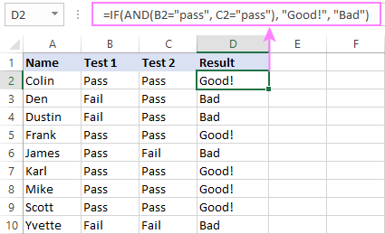
Important note! The AND function checks all the conditions, even if the already tested one(s) evaluated to FALSE. Such behavior is a bit unusual since in most of programming languages, subsequent conditions are not tested if any of the previous tests has returned FALSE.
In practice, a seemingly correct IF statement may result in an error because of this specificity. For example, the below formula would return #DIV/0! ("divide by zero" error) if cell A2 is equal to 0:
=IF(AND(A2<>0, (1/A2)>0.5),"Good", "Bad")
The avoid this, you should use a nested IF function:
=IF(A2<>0, IF((1/A2)>0.5, "Good", "Bad"), "Bad")
For more information, please see IF AND formula in Excel.
Excel IF function with multiple conditions (OR logic)
To do one thing if any condition is met, otherwise do something else, use this combination of the IF and OR functions:
The difference from the IF / AND formula discussed above is that Excel returns TRUE if any of the specified conditions is true.
So, if in the previous formula, we use OR instead of AND:
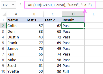
=IF(OR(B2>50, B2>50), "Pass", "Fail")
Then anyone who has more than 50 points in either exam will get "Pass" in column D. With such conditions, our students have a better chance to pass the final exam (Yvette being particularly unlucky failing by just 1 point :)
Tip. In case you are creating a multiple IF statement with text and testing a value in one cell with the OR logic (i.e. a cell can be "this" or "that"), then you can build a more compact formula using an array constant.
For example, to mark a sale as "closed" if cell B2 is either "delivered" or "paid", the formula is:
=IF(OR(B2={"delivered", "paid"}), "Closed", "")
More formula examples can be found in Excel IF OR function.
IF with multiple AND & OR statements
If your task requires evaluating several sets of multiple conditions, you will have to utilize both AND & OR functions at a time.
In our sample table, suppose you have the following criteria for checking the exam results:
- Condition 1: exam1>50 and exam2>50
- Condition 2: exam1>40 and exam2>60
If either of the conditions is met, the final exam is deemed passed.
At first sight, the formula seems a little tricky, but in fact it is not! You just express each of the above conditions as an AND statement and nest them in the OR function (since it's not necessary to meet both conditions, either will suffice):
OR(AND(B2>50, C2>50), AND(B2>40, C2>60)
Then, use the OR function for the logical test of IF and supply the desired value_if_true and value_if_false values. As the result, you get the following IF formula with multiple AND / OR conditions:
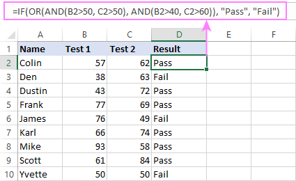
=IF(OR(AND(B2>50, C2>50), AND(B2>40, C2>60), "Pass", "Fail")
The screenshot below indicates that we've done the formula right:
Naturally, you are not limited to using only two AND/OR functions in your IF formulas. You can use as many of them as your business logic requires, provided that:
- In Excel 2007 and higher, you have no more than 255 arguments, and the total length of the IF formula does not exceed 8,192 characters.
- In Excel 2003 and lower, there are no more than 30 arguments, and the total length of your IF formula does not exceed 1,024 characters.
Nested IF statement to check multiple logical tests
If you want to evaluate multiple logical tests within a single formula, then you can nest several functions one into another. Such functions are called nested IF functions. They prove particularly useful when you wish to return different values depending on the logical tests' results.
Here's a typical example: suppose you want to qualify the students' achievements as "Good", "Satisfactory" and "Poor" based on the following scores:
- Good: 60 or more (>=60)
- Satisfactory: between 40 and 60 (>40 and <60)
- Poor: 40 or less (<=40)
Before writing a formula, consider the order of functions you are going to nest. Excel will evaluate the logical tests in the order they appear in the formula. Once a condition evaluates to TRUE, the subsequent conditions are not tested, meaning the formula stops after the first TRUE result.
In our case, the functions are arranged from largest to smallest:
=IF(B2>=60, "Good", IF(B2>40, "Satisfactory", "Poor"))
Naturally, you can nest more functions if needed (up to 64 in modern versions).

For more information, please see How to use multiple nested IF statements in Excel.
Excel IF array formula with multiple conditions
Another way to get an Excel IF to test multiple conditions is by using an array formula.
To evaluate conditions with the AND logic, use the asterisk:
To test conditions with the OR logic, use the plus sign:
To complete an array formula correctly, press the Ctrl + Shift + Enter keys together. In Excel 365 and Excel 2021, this also works as a regular formula due to support for dynamic arrays.
For example, to get "Pass" if both B2 and C2 are greater than 50, the formula is:
=IF((B2>50) * (C2>50), "Pass", "Fail")

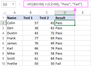
In my Excel 365, a normal formula works just fine (as you can see in the screenshots above). In Excel 2019 and lower, remember to make it an array formula by using the Ctrl + Shift + Enter shortcut.
To evaluate multiple conditions with the OR logic, the formula is:
=IF((B2>50) + (C2>50), "Pass", "Fail")
Using IF together with other functions
This section explains how to use IF in combination with other Excel functions and what benefits this gives to you.
Example 1. If #N/A error in VLOOKUP
When VLOOKUP or other lookup function cannot find something, it returns a #N/A error. To make your tables look nicer, you can return zero, blank, or specific text if #N/A. For this, use this generic formula:
For example:
If #N/A return 0:
If the lookup value in E1 is not found, the formula returns zero.
=IF(ISNA(VLOOKUP(E1, A2:B10, 2,FALSE )), 0, VLOOKUP(E1, A2:B10, 2, FALSE))
If #N/A return blank:
If the lookup value is not found, the formula returns nothing (an empty string).
=IF(ISNA(VLOOKUP(E1, A2:B10, 2,FALSE )), "", VLOOKUP(E1, A2:B10, 2, FALSE))
If #N/A return certain text:
If the lookup value is not found, the formula returns specific text.
=IF(ISNA(VLOOKUP(E1, A2:B10, 2,FALSE )), "Not found", VLOOKUP(E1, A2:B10, 2, FALSE))

For more formula examples, please see VLOOKUP with IF statement in Excel.
Example 2. IF with SUM, AVERAGE, MIN and MAX functions
To sum cell values based on certain criteria, Excel provides the SUMIF and SUMIFS functions.
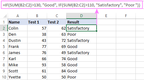
In some situations, your business logic may require including the SUM function in the logical test of IF. For example, to return different text labels depending on the sum of the values in B2 and C2, the formula is:
=IF(SUM(B2:C2)>130, "Good", IF(SUM(B2:C2)>110, "Satisfactory", "Poor"))
If the sum is greater than 130, the result is "good"; if greater than 110 – "satisfactory', if 110 or lower – "poor".
In a similar fashion, you can embed the AVERAGE function in the logical test of IF and return different labels based on the average score:
=IF(AVERAGE(B2:C2)>65, "Good", IF(AVERAGE(B2:C2)>55, "Satisfactory", "Poor"))
Assuming the total score is in column D, you can identify the highest and lowest values with the help of the MAX and MIN functions:
=IF(D2=MAX($D$2:$D$10), "Best result", "")
=IF(D2=MAX($D$2:$D$10), "Best result", "")
To have both labels in one column, nest the above functions one into another:
=IF(D2=MAX($D$2:$D$10), "Best result", IF(D2=MIN($D$2:$D$10), "Worst result", ""))

Likewise, you can use IF together with your custom functions. For example, you can combine it with GetCellColor or GetCellFontColor to return different results based on a cell color.
In addition, Excel provides a number of functions to calculate data based on conditions. For detailed formula examples, please check out the following tutorials:
Example 3. IF with ISNUMBER, ISTEXT and ISBLANK
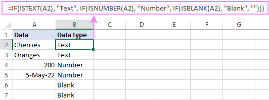
To identify text, numbers and blank cells, Microsoft Excel provides special functions such as ISTEXT, ISNUMBER and ISBLANK. By placing them in the logical tests of three nested IF statements, you can identify all different data types in one go:
=IF(ISTEXT(A2), "Text", IF(ISNUMBER(A2), "Number", IF(ISBLANK(A2), "Blank", "")))
Example 4. IF and CONCATENATE
To output the result of IF and some text into one cell, use the CONCATENATE or CONCAT (in Excel 2016 - 365) and IF functions together. For example:
=CONCATENATE("You performed ", IF(B1>100,"fantastic!", IF(B1>50, "well", "poor")))
=CONCAT("You performed ", IF(B1>100,"fantastic!", IF(B1>50, "well", "poor")))
Looking at the screenshot below, you'll hardly need any explanation of what the formula does:

IF ISERROR / ISNA formula in Excel
The modern versions of Excel have special functions to trap errors and replace them with another calculation or predefined value - IFERROR (in Excel 2007 and later) and IFNA (in Excel 2013 and later). In earlier Excel versions, you can use the IF ISERROR and IF ISNA combinations instead.
The difference is that IFERROR and ISERROR handle all possible Excel errors, including #VALUE!, #N/A, #NAME?, #REF!, #NUM!, #DIV/0!, and #NULL!. While IFNA and ISNA specialize solely in #N/A errors.
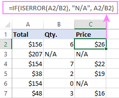
For example, to replace the "divide by zero" error (#DIV/0!) with your custom text, you can use the following formula:
=IF(ISERROR(A2/B2), "N/A", A2/B2)
And that's all I have to say about using the IF function in Excel. I thank you for reading and hope to see you on our blog next week!
Practice workbook for download
Excel IF multiple criteria - examples (.xlsx file)
 by
by
4506 comments
Hi Friends
Could you please help me to get the excel formula for the below mentioned calculation.
If value of cell(say X)<10 then value is 5,if X in between 10 to 100 then value is 0.7%*X & minimum value 6,
if X in between 100 to 200 then value is 0.6%*X & minimum value is 7 and maximum value is 9.
Looking forward for your kind support & thank you in advance.
Thanks & Reagrds
Aman Kumar
Hi Friends
Could you please help me to get the excel formula for the below mentioned calculation.
If value of cell(say X)<10 then value is 5,if X in between 10 to 100 then value is 0.7%*X & minimum value 6,
if X in between 100 to 200 then value is 0.6%*X & minimum value is 7 and maximum value is 9.
Looking forward for your kind support & thank you in advance.
Thanks & Regards
Aman Kumar
Hi please help me. I've been cracking my head for almost a week now.I need a formula to sum up this
If column is 1 then multiply with 0.65
If column is 2 then multiply with 0.55
If column is 3 then multiply with 0.45
If column is 4 then multiply with 0.35
=IF(A1=1,A1*0.65,IF(A1=2,A1*0.55,IF(A1=3,A1*0.45,A1*0.35)))
Hi,
I need your advice. I can't find a way to write a formula for multiple logic from 2 different cells.
To determine "Moving" from one of the cell, let's say A1 is "Yes".
To determine "Sales" from one of cell, B1 is any number more than "0".
Here are the logic:
1. With Moving & With Sales = Moving
2. Without Moving & without Sales = Non-moving
3. With Moving & Without Sales = Others
4. Without Moving & With Sales = Others
So, what should I put C1 for the formula.
I tried combination of IF (AND & OR) but failed.
=IF(AND(E2="Yes";G2>=1);"Moving";"")&IF(AND(E2="No";G2=0);"Non-moving";"")&IF(AND(E2="Yes";G2=0);"Others";"")&IF(AND(E2="No";G2=0);"Others";"")
It ended up with 2 results in 1 cell. For example, Non-moving & Others.
Please help.
Thank you so much!
I managed to solve it.
=IF(AND(E17="Yes";G17>=1);"Moving";"")&IF(AND(E17="No";G17=0);"Non-moving";"")&IF(AND(E17="Yes";G17=0);"Others";"")&IF(AND(E17="No";G17>=1);"Others";"")
Hi,
I need your advice. I can't find a way to write a formula for multiple logic from 2 different cells.
To determine "Moving" from one of the cell, let's say A1 is "Yes".
To determine "Sales" from one of cell, B1 is any number more than "0".
Here are the logic:
1. With Moving & With Sales = Moving
2. Without Moving & without Sales = Non-moving
3. With Moving & Without Sales = Others
4. Without Moving & With Sales = Others
So, what should I put C1 for the formula.
I tried combination of IF (AND & OR) but failed.
Please help.
Thank you so much!
Hi there, I can't find a way to write a formula. I have the following list and I want in A6 write the number form B if A5 in the A list
| A | B |
1|aaa| 4 |
2|bbb| 2 |
3|ccc| 8 |
If A5=aaa then write 4, If A5=bbb then write 2, If A5=ccc then write 8
Thank you
Hi there,
I have a problem to be solved. like,
Leave
Taken CL SL PL CL2 SL2 PL2
0 0.5 0.5 22
10 0.5 0.5 3.5
2 0.5 0.5 2
0 0.5 0.5 6.5
4 0.5 0.5 43.5
i want to have a formula if cl2 leave taken than shud be = number(value)
or if cl2=leave taken than shud be =0. can we do that. please advise.
Hi I want to creates system that assigns roll numbers to my students.
the conditions are:
if 1-99 then it should display roll as SA followed by the number eg roll assignment should be SA1 for the 1st student, SA2 for 2nd student etc.
For the next 100-999 then it should display roll as SB1 for the 100th student,SB2 for the 101st student.
Hello Lavanya,
If you have serial numbers from 1 to 999 in some column, say column A, you can use the following formula:
=IF(A1>99, "SB"&A1-99, IF(A1>0, "SA"&A1, ""))
Or, you can generate roll numbers based on the row numbers in a worksheet:
=IF(ROW()>99, "SB"&ROW()-99, "SA"&ROW())
in ecxellsheet 1 column of date,i want that date become red when diff between today date and that day is above 365 day...which formula i used???
Hi,
I need some help how to create a formula that combines 2 sheets in my work book.
I need formula to do this: If "name" in under some specific "date" then I want the "value" that is in cell next to to the "name" and under that "date" to be transferred to a cell under the same "date" but in other sheet.
Can this be done and if it can how?
Very much appreciate any help you can provide on this matter.
Thank you in advance.
Sincerely yours,
Eduard
Hello Ms. Svetlana,
I am using advance filters (and data range w/ drop down list) to filter data from a table with projects information, including "End Date" (of the project). The problem is, I have numbers (date) and sometimes text (e.x. "ongoing" project) in the cell, so the advance filter doesn´t work. I think I need a "If" statment that works with both numbers and text in the same cell.
Thanks for your time!
Hello,
I want give range in if condition
=IF(A2:A17=I2:I14,"Match","Not Match")
i have a column whose name "A" and same as "I" i want to compare his value.
i want to match entire "A" and "I" column's value.
is it possible then please guide me....
Hi, could you help to set up a formula for below question?
Q: >=1000kg, 0.1/kg; >=2000kg,0.09/kg; >=3000kg,0.08kg, Min.100, Max.500.
Thanks a lot.
Hi
I am trying to do a formula in excel which looks up a date from a cell in one sheet in to the equivalent cell in another sheet, however I have a couple scenarios that are a problem. I am looking up 2 columns both of which have dates in them, in the first column I need to look up F2 from one sheet and put it in to the other sheet in F2, however I have some blanks so I have used an ISBLANK formula without a problem =IF(ISBLANK('MAIN LIST 2'!F2)," ",('MAIN LIST 2'!F2)).
I also have to look up G2 from one sheet to the other equivalent cell, however if there is a blank in cell G2, I need to use what is in F2 which I have used =IF('MAIN LIST 2'!G2,'MAIN LIST 2'!G2,'MAIN LIST 2'!F2), however this brings back 00/01/1900 in some cells where the cells in column F is blank. How do I return a blank in G2 if both F2 and G2 are both blank in the other sheet.
Thanks
Hai,
Please help me to get a formula for my payroll calculation.Conditions are if an employee need to present for only 24 days in a month his salary will be the basic salary and if he comes more than the required days in a month ,ie, in this month more than 24 days his salary will be basic salary + basic salary/26*additional days present and if he is present for less than required days, no salary deducted for 2 grace days but if it is less than 22 days in this month his salary will be basic salary minus (basic salary/26*(22-number of attendance)
Hi,
could you tell me what is wrong with the formula below?
it does not work for routine
=IF(AND(H2="emergency",N2>TIME(3,0,0)),"Failed",IF(AND(H2="emergency",L2>TIME(0,20,0)),"Failed",IF(AND(H2="urgent",N2>TIME(24,0,0)),"Failed",IF(AND(H2="urgent",L2>TIME(4,0,0)),"Failed",IF(AND(H2="routine",N2>TIME(72,0,0)),"Failed",IF(AND(H2="routine",L2>TIME(24,0,0)),"Failed","Passed"))))))
=IF(E6="S",IF(G4>=3,"PAID",IF(G4=0,"DUE","PART PAYMENT")))
+
IF(E6="F",IF(G4>=6,"PAID",IF(G4=0,"DUE","PART PAYMENT")))
I want to merge this two formula
Hi, i wish you could help me with this problem,
Cell A is due date
Cell B is invoice amount
Cell C is Amount paid
Cell D is Open Balance
Cell E is status
I would like to put formulae in cell E to have either paid,overdue or open.
Hi, I am having problems trying to come up for a formula for the following:
Amount Service Count
1 0.00% 1
1 100% 0
2 50% 1
4 50% 2
So, If service is 0% the count should be the contents of amount, if 100% the count should be equal to zero but if the service is 50% it should be the 50% of the contents of the amount cell.
Please help my on this formula
I want every cell in the row more than 60 to give me the difference otherwise if it is 60 than give me a 0
My formula looks like:
=IF('TOTAL WEEK 1'!$D$4:$R$4>60;'TOTAL WEEK 1'!$D$4:$R$4-60;0)
But if give me only a result if it is more in the first cell not in the following cells .
Thank you in advance
Hi there I cant work out how to do this function:
If H39 is between 0 and 50000 * 0.1. if H39 is between 50000 and 100000 *0.085. if H39 is between 100000 and 500000 *0.06. if H39 is over 500000 *0.05
are you able to help
thanks
Hello,
Please help, I need formula for below condition:
If 0-30 should show "C", if 31-60 should show "B", if 61 above should show "C".
Thanks
Hello!
Here you go:
=IF(AND(A1>=0,A1<31), "C", IF(A1<61,"B", "A"))
Please note that your conditions have "C" for 0-30, and >61, which is obviously a misprint, so I used "A" for the latter.
Pl send me formula for below criteria.
New Hires
Individuals, who join on or before the 10th of any month, will earn MTO credit for the period from the 1st to the 15th of the month and accrue such credit on the 16th of the month. Individuals, who join after the 10th of the month, will not earn any MTO credit on the 16th of the month.
Individuals, who join on or before the 25th of any month, will earn MTO credit for the period from the 16th to the end of the month on the 1st of the following month. Individuals, who join after the 25th of the month, will not earn any MTO credits on the 1st of the following month.
Separations
Individuals, who leave the services of the company on or after the 10th of any month, will earn MTO credit for the period from the 1st to the 15th of such month. Individuals, who leave before the 10th of the month, will not earn any MTO credits for the period from the 1st to the 15th of such month.
Individuals, who leave the services of the company on or after the 25th of any month, will earn MTO credit for the period from the 16th to the end of such month. Individuals, who leave before the 25th of the month, will not earn any MTO credits for the period from the 16th to the end of such month.
=IF(B3>69,20(OR(B3>50403010<29,2))))))))). Not sure my formula showed up completely.
Hello Barbara,
It looks like the formula got posted all wrong, sorry for this. Can you please describe the conditions in words?
For example:
- If B3 is greater than 69, return 20
- If B3 is greater than 50, then what? etc.
If b3 is greater than 69, return 20
If b3 is greater than 50, less than 68, return 15
If be is greater than 40, less than 49, return 10
If b is greater than 30, less than 48, return 5
If b3 is less than 29, return 2
I hope this one is more clear. Thank you Svetlana
Hello Barbara,
You can us the following nested If's:
=IF(B3>69,20, IF(B3>=50,15, IF(B3>=40,10, IF(B3>=30,5,2))))
=IF(B3>69,20,(OR(B3>50403010<29,2)))))))))
This formula is supposed to give me a hard number (20, 15, 10, 5, 0) based on the based upon input in b3. The first statement works correctly and returns a 20 if >69 in b3, however, the remainder of the formula returns "True" rather than a number. Can you tell me what I am doing wrong? Thank you.
Hi,
I'm new to this but want to do the following:
if cell D11 is 6 then then the payment is £450 plus £60 for each additional number
ie. 9 people attended = £450 + (3*60) = £630
Can anyone help?
Thanks in advance
Sorry but some of my original message went AWOL.
if D11 is 6 = £450 + £60 for each additional number (ie 9 people attended = £450 + (3*60) = £630
Thanks
Hi Alison,
If my understanding of the task is correct, the following formula should work a treat:
=IF(D11=6, 450, 450+(60*(D11-6)))
How can i replace an number to an text
Exmaple:
If i type 1 in an box and press enter. The text in the box will be replaced with "hey"
I type 1 and this is the output:
____________
|___hey____|
Hi ,
I want formula for the below.
Define buckets based on the below logic
Bucket C – Less than 2 week from today
Bucket D – More than 2 weeks and less than 1 month from today
Bucket E – More than 1 month and less than 3 months from today
Bucket F – More than 3 months and less than 6 months from today
Bucket G – More than 6 months and less than 12 months from today
Bucket H – More than 12 months and less than 2 years from today
Bucket I – More than 2 years and less than 5 years from today
Bucket J – More than 5 years from today
I'm trying to work out commission structures in excel, for example if the fee is between 25k-49.99k, then the commission is 1.25%, if fee is between 50k-99.99k then commission is 1%, if fee is between 1 lacs - 199.99 lacs then commission is 0.75%, if fee is 2 lacs and above commission is 0.5%
awesome post. very helpful!!
Hi Svetlana,
I want to calculate the difference between date 1 "I3" and date 2 "L3", but in case of date 2 "L3" not available I want to calculate it between 1 "I3" and today date so, I wrote this formula but I keep receiving wrong result cause of not applying today formula
=IF(L3,"=(TODAY())-(I3)",(L3-I3))
Hi Muahammad,
Try this formula:
=IF(L3="", TODAY()-I3, L3-I3)
Thank you!! Your article is super clear! I had never understood the logic behind this functions until now.
I'm trying to find the max excluding the middle portions of the data set. Using the table below, i'd like to find the max above Time=7 and below time=4. I've tried various permutations
Time Total
1 0
2 0
3 12
4 0
5 20
6 19
7 0
8 11
9 0
10 0
I think =MAX(IF(OR(A2:A11>7,A2:A11<4),B2:B11)) should work but it just returns the max of the entire data set (ie 20). If i break up the formula (ie exclude the OR) and add a secondary step it works. Any tips?
Hi!
This is my current formula: =if(and(ISBLANK(F2),ISTEXT(G2)),"New",)
Right now, if there is no text in F2 AND there is text in G2, the cell will say "New"
I want to add to the formula so it's this way:
If there is no text in F2 AND there is text in G2, the cell will say "New" but IF there is text in G2 and F2, the cell should say "Ad Proofing"
Could someone help me with this? Thank you!
=if(and(ISBLANK(F2),ISTEXT(G2)),"New","Add Proofing") try this should help
I would like to add multiple conditions to my spreadsheet for example: for every A.. that has "name" and B.. that has 1 then add 0.05 to G1
Dear Sir,
How can use over 9 conditions.
=IF(H11=2,I19+H19+H20+H21,IF(H11=3,I20+H20+H21,IF(H11=4,I21+H21+H22,IF(H11=5,I22+H22+H23,IF(H11=6,I23+H23+H24,IF(H11=7,I24+H24+H25,IF(H11=8,I25+H25+H26,IF(H11=9,I26+H26+H27))))))))
It may have to do with the version of Excel you are using. If it is an older version, I believe you can only have a maximum of 7 conditions. The newer versions allow up to 64. You may want to look into that.
hie.
l still need help my formula isn't giving me an answer
l'm still having problems with finding grade using the average mark
l need help on calculating grade using average mark.l used =if(average (B2:G2)>75,"A",if(average (B2:G2)>60,"B",if(average(B2:G2)>50,"C",if(average(B2:G2)>45,"D",if(average(B2:G2)>40,"E","U"))))).It says there is an error in my formula.please help.
hi,
i want a formula so that i come to know that if a particular cheque issued then amount of that cheque will appear in next cell,
for example
AMOUNT CHQ NO STATUS DATE OF ISSUE DATE OF CLEARENCE Amount(if cleared)
2977 54808 issued 21.04.2016 25.04.2016
as above mentioned i want to next cell which is blank shows the amount if a particular cheque has cleared from bank and also i've given the clearance date of cheque
please guid
Thanx & Regards
Ghayas Ahmad
I am trying to make an If then statement for the following:
If box F5 = 100, then box F6 = 3000
if box F5 100, then box F6 = 5 x every number over 100 + 3000
(example if F5 = 105, the box F6 would need to be (5*5)+3000
Could you help me make a formula? Please?
it cut off part of my formula:
also add in: if box F5 < 100, than F6 = 3000
Hi Emily,
Try the following formula:
=IF(F5<=100, 3000, 5*(F5-100)+3000)
I have a spreadsheet that has a due date in column j, and a status of open or closed in column K.
I need Column L to calculate if the date is after today's date, and the status is open, then it says On Track, if the date is after today's date and the status is closed, then it says completed, and if the date is before today's date and the status is either open or closed then it shows Delayed... I've figured out how to get it to show On Track, Completed and Delayed based on just the date in column j, but I can't figure out how to get the status involved.
Hi Kayla,
Please use the below function,
=IF(AND(J14>TODAY(),K14="Open"),"On Track",IF(AND(J14>TODAY(),K14="Close"),"Completed",IF(AND(J14<TODAY(),OR(K14="Open",K14="Close")),"Delayed","")))
Thanks,
Prabath
Hi,
I have scenario,
I am trying to get all the blank fields from the column, for ex- if I have this column.
13 years 6 months 0 days
34 years 5 months 0 days
10 years 9 months 0 days
14 years 0 days
6 years 8 months 0 days
5 years 11 months 0 days
23 years 6 months
6 years 9 months 0 days
8 years 9 months 0 days
30 years 9 months 0 days
7 years 7 months 0 days
15 years 4 months 0 days
45 years 3 months 0 days
40 years 10 months 0 days
33 years 2 months 0 days
13 years 9 months 0 days
30 years 2 months 0 days
29 years 10 months 0 days
25 years 6 months 0 days
14 years 9 months 0 days
41 years 3 months 0 days
10 years 11 months 0 days
30 years 3 months 0 days
15 years 11 months 0 days
27 years 0 days 6 years
As you can the column has the blank fields, I need to get the blank fields out from the column, also it has "NUM" error and 0, which I also need need to take out.
Can you please tell me how to construct the formula for that.
Thanks,
Saurabh
Hello Saurabh,
I recommend you to use filter. So you can select blank rows and remove them.
https://support.office.com/en-us/article/Add-or-remove-table-rows-and-columns-in-an-Excel-table-4d6585be-4292-444c-b86b-71cb4e5d3e16#bmremoveblankrows
Similarly you can choose the rows with errors and remove them.
Hi can you help me with the conditions for this !
If age is between 0 - 12 months then 0.5 to 1.8 µmol/L
If age is between 1 - 6 years: then 0.7 to 1.5 µmol/L
If age is between 7 - 12 years: then 0.9 to 1.7 µmol/L
If age is between 13 - 18 years:then 0.9 to 2.5 µmol/L
If age is ≥ 18 years:then 1.5 - 3.5 µmol/L
Hi,
use this function,
=IF(A2<1,"0.5 to 1.8 umol/L",IF(A2<6,"0.7 to 1.5 umol/L",IF(A2<12,"0.9 to 1.7 umol/L",IF(A2<18,"0.9 to 2.5 umol/L","1.5 to 3.5 umol/L"))))
Thanks,
Prabath
Hi Sam!
Use the following formula to calculate a months count
=(YEAR(NOW())-YEAR(A1))*12+MONTH(NOW())-MONTH(A1)
So your formula is:
=IF((YEAR(NOW())-YEAR(A1))*12+MONTH(NOW())-MONTH(A1)>18*12,"1.5 - 3.5 µmol/L",IF((YEAR(NOW())-YEAR(A1))*12+MONTH(NOW())-MONTH(A1)>13*12,"0.9 to 2.5 µmol/L",IF((YEAR(NOW())-YEAR(A1))*12+MONTH(NOW())-MONTH(A1)>7*12,"0.9 - 1.7 µmol/L",IF((YEAR(NOW())-YEAR(A1))*12+MONTH(NOW())-MONTH(A1)>1*12,"0.7 - 1.5 µmol/L","0.5 to 1.8 µmol/L"))))
Please note A1 should be contain a birth date.
Hi,
If above once is not clear. Please assist me by using this one.
Invoice # Value
MYEX0455477 10.00
MYEX0456058 5.00
MYAE0154262 8.00
MYEX0456603 8.00
MYEX0456601 7.00
MYAE0154534 2.00
MYEX0457138 11.00
MYEX0457438 9.00
MYAI0069730 14.00
MYEX0457318 6.00
Matching Amount 20.00
Combinations
MYEX0455477 10.00
MYAE0154262 8.00
MYAE0154534 2.00 20.00
MYEX0455477 10.00
MYEX0456603 8.00
MYAE0154534 2.00 20.00
MYEX0456058 5.00
MYAE0154262 8.00
MYEX0456601 7.00 20.00
MYEX0456058 5.00
MYEX0456603 8.00
MYEX0456601 7.00 20.00
MYEX0457138 11.00
MYEX0457438 9.00 20.00
MYAI0069730 14.00
MYEX0457318 6.00 20.00
Thanks,
Regards,
Prabath
Hi all,
I have 10 Invoices & 10 Invoice value as below. I want to get all possible combinations of Invoices which value is equal to 20. How is it possible to get it by using excel? I have mentioned the possible combination for easy reference.
Invoice # Value Matching Amount 20
MYEX0455477 10 Combinations
MYEX0456058 5
MYAE0154262 8 MYEX0455477 10
MYEX0456603 8 MYAE0154262 8
MYEX0456601 7 MYAE0154534 2 20
MYAE0154534 2
MYEX0457138 11 MYEX0455477 10
MYEX0457438 9 MYEX0456603 8
MYAI0069730 14 MYAE0154534 2 20
MYEX0457318 6
MYEX0456058 5
MYAE0154262 8
MYEX0456601 7 20
MYEX0456058 5
MYEX0456603 8
MYEX0456601 7 20
MYEX0457138 11
MYEX0457438 9 20
MYAI0069730 14
MYEX0457318 6 20
Thank you,
Regards,
Prabath
Hi Svetlana,
I need some help on below issue.
Below function has been created to get the status of Customer Statement of Account as mentioned below. As per my function, If there are no details in C4, I'm getting the status as "Unapplied". But I need it to be zero. How can I write this function.
=IF(RIGHT(C4,1)="I","Invoice",IF(RIGHT(C4,1)="C","Credit Note",IF(AND(C4="NULL",A4="Unidentified"),"Unidentified","Unapplied")))
Thanks for you guidance in all the time.
Thank You,
Regards,
Prabath
Hi Prabath,
If "no details in C4" means "if C4 is blank", then you can simply add one more IF statement to your formula:
=IF(C4="", 0, IF(RIGHT(C4,1)="I","Invoice",IF(RIGHT(C4,1)="C","Credit Note",IF(AND(C4="NULL",A4="Unidentified"),"Unidentified","Unapplied"))))
Hi Svetlana,
Thank you very much. This is exactly what i want.
Thanks,
Regards,
Prabath
Good afternoon,
how could i round down a number when its decimals are smaller than 0,5 and if not it stays the same?
Hi Bocirnea,
Please use this function,
=ROUNDDOWN(B3,1)
Thanks,
Regards,
Prabath
Hi there, how can I make this less complicated or shorter. If a cell is =IF(OR(A1=B1:B250,C1,IF(A1=B251:265,C2))
CURRENTLY I HAVE IT AS - =IF(F6=D217,A285,IF(F6=D218,A285,IF(F6=D219,A285,IF(F6=D220,A285,IF(F6=D221,A285,IF(F6=D222,A285,IF(F6=D223,A285,IF(F6=D224,A285,IF(F6=D225,A285,IF(F6=D226,A285,IF(F6=D227,A285,IF(F6=D228,A285,IF(F6=D229,A285,IF(F6=D230,A285,IF(F6=D231,A285,IF(F6=D232,A285,IF(F6=D233,A285,IF(F6=D234,A285,IF(F6=D235,A285,IF(F6=D236,A285,IF(F6=D237,A285,IF(F6=D238,A285,IF(F6=D239,A285,IF(F6=D240,A285,IF(F6=D241,A285,IF(F6=D242,A285,IF(F6=D243,A285,IF(F6=D244,A285,IF(F6=D245,A285,IF(F6=D246,A285,IF(F6=D247,A285,IF(F6=D248,A285,IF(F6=D249,A285,IF(F6=D250,A285,IF(F6=D251,A285,IF(F6=D252,A285,IF(F6=D253,A286,IF(F6=D254,A286,IF(F6=D255,A286,IF(F6=D256,A286,IF(F6=D257,A286,IF(F6=D258,A286,IF(F6=D259,A286,IF(F6=D260,A286,IF(F6=D261,A286,IF(F6=D262,A286))))))))))))))))))))))))))))))))))))))))))))))