The tutorial shows how to create multiple IF statements in Excel with AND as well as OR logic. Also, you will learn how to use IF together with other Excel functions.
In the first part of our Excel IF tutorial, we looked at how to construct a simple IF statement with one condition for text, numbers, dates, blanks and non-blanks. For powerful data analysis, however, you may often need to evaluate multiple conditions at a time. The below formula examples will show you the most effective ways to do this.
How to use IF function with multiple conditions
In essence, there are two types of the IF formula with multiple criteria based on the AND / OR logic. Consequently, in the logical test of your IF formula, you should use one of these functions:
- AND function - returns TRUE if all the conditions are met; FALSE otherwise.
- OR function - returns TRUE if any single condition is met; FALSE otherwise.
To better illustrate the point, let's investigate some real-life formulas examples.
Excel IF statement with multiple conditions (AND logic)
The generic formula of Excel IF with two or more conditions is this:
Translated into a human language, the formula says: If condition 1 is true AND condition 2 is true, return value_if_true; else return value_if_false.
Suppose you have a table listing the scores of two tests in columns B and C. To pass the final exam, a student must have both scores greater than 50.
For the logical test, you use the following AND statement: AND(B2>50, C2>50)
If both conditions are true, the formula will return "Pass"; if any condition is false - "Fail".
=IF(AND(B2>50, B2>50), "Pass", "Fail")
Easy, isn't it? The screenshot below proves that our Excel IF /AND formula works right:

In a similar manner, you can use the Excel IF function with multiple text conditions.
For instance, to output "Good" if both B2 and C2 are greater than 50, "Bad" otherwise, the formula is:
=IF(AND(B2="pass", C2="pass"), "Good!", "Bad")
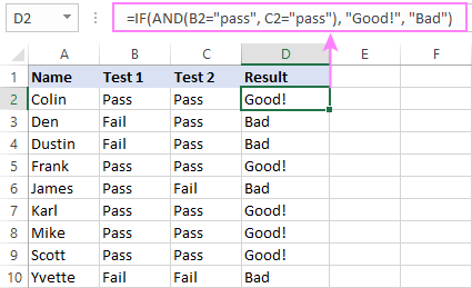
Important note! The AND function checks all the conditions, even if the already tested one(s) evaluated to FALSE. Such behavior is a bit unusual since in most of programming languages, subsequent conditions are not tested if any of the previous tests has returned FALSE.
In practice, a seemingly correct IF statement may result in an error because of this specificity. For example, the below formula would return #DIV/0! ("divide by zero" error) if cell A2 is equal to 0:
=IF(AND(A2<>0, (1/A2)>0.5),"Good", "Bad")
The avoid this, you should use a nested IF function:
=IF(A2<>0, IF((1/A2)>0.5, "Good", "Bad"), "Bad")
For more information, please see IF AND formula in Excel.
Excel IF function with multiple conditions (OR logic)
To do one thing if any condition is met, otherwise do something else, use this combination of the IF and OR functions:
The difference from the IF / AND formula discussed above is that Excel returns TRUE if any of the specified conditions is true.
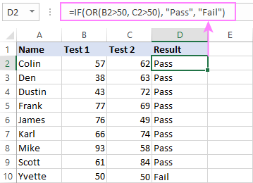
So, if in the previous formula, we use OR instead of AND:
=IF(OR(B2>50, B2>50), "Pass", "Fail")
Then anyone who has more than 50 points in either exam will get "Pass" in column D. With such conditions, our students have a better chance to pass the final exam (Yvette being particularly unlucky failing by just 1 point :)
Tip. In case you are creating a multiple IF statement with text and testing a value in one cell with the OR logic (i.e. a cell can be "this" or "that"), then you can build a more compact formula using an array constant.
For example, to mark a sale as "closed" if cell B2 is either "delivered" or "paid", the formula is:
=IF(OR(B2={"delivered", "paid"}), "Closed", "")
More formula examples can be found in Excel IF OR function.
IF with multiple AND & OR statements
If your task requires evaluating several sets of multiple conditions, you will have to utilize both AND & OR functions at a time.
In our sample table, suppose you have the following criteria for checking the exam results:
- Condition 1: exam1>50 and exam2>50
- Condition 2: exam1>40 and exam2>60
If either of the conditions is met, the final exam is deemed passed.
At first sight, the formula seems a little tricky, but in fact it is not! You just express each of the above conditions as an AND statement and nest them in the OR function (since it's not necessary to meet both conditions, either will suffice):
OR(AND(B2>50, C2>50), AND(B2>40, C2>60)
Then, use the OR function for the logical test of IF and supply the desired value_if_true and value_if_false values. As the result, you get the following IF formula with multiple AND / OR conditions:
=IF(OR(AND(B2>50, C2>50), AND(B2>40, C2>60), "Pass", "Fail")
The screenshot below indicates that we've done the formula right:
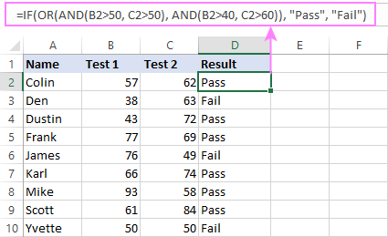
Naturally, you are not limited to using only two AND/OR functions in your IF formulas. You can use as many of them as your business logic requires, provided that:
- In Excel 2007 and higher, you have no more than 255 arguments, and the total length of the IF formula does not exceed 8,192 characters.
- In Excel 2003 and lower, there are no more than 30 arguments, and the total length of your IF formula does not exceed 1,024 characters.
Nested IF statement to check multiple logical tests
If you want to evaluate multiple logical tests within a single formula, then you can nest several functions one into another. Such functions are called nested IF functions. They prove particularly useful when you wish to return different values depending on the logical tests' results.
Here's a typical example: suppose you want to qualify the students' achievements as "Good", "Satisfactory" and "Poor" based on the following scores:
- Good: 60 or more (>=60)
- Satisfactory: between 40 and 60 (>40 and <60)
- Poor: 40 or less (<=40)
Before writing a formula, consider the order of functions you are going to nest. Excel will evaluate the logical tests in the order they appear in the formula. Once a condition evaluates to TRUE, the subsequent conditions are not tested, meaning the formula stops after the first TRUE result.
In our case, the functions are arranged from largest to smallest:
=IF(B2>=60, "Good", IF(B2>40, "Satisfactory", "Poor"))
Naturally, you can nest more functions if needed (up to 64 in modern versions).

For more information, please see How to use multiple nested IF statements in Excel.
Excel IF array formula with multiple conditions
Another way to get an Excel IF to test multiple conditions is by using an array formula.
To evaluate conditions with the AND logic, use the asterisk:
To test conditions with the OR logic, use the plus sign:
To complete an array formula correctly, press the Ctrl + Shift + Enter keys together. In Excel 365 and Excel 2021, this also works as a regular formula due to support for dynamic arrays.
For example, to get "Pass" if both B2 and C2 are greater than 50, the formula is:
=IF((B2>50) * (C2>50), "Pass", "Fail")

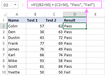
In my Excel 365, a normal formula works just fine (as you can see in the screenshots above). In Excel 2019 and lower, remember to make it an array formula by using the Ctrl + Shift + Enter shortcut.
To evaluate multiple conditions with the OR logic, the formula is:
=IF((B2>50) + (C2>50), "Pass", "Fail")
Using IF together with other functions
This section explains how to use IF in combination with other Excel functions and what benefits this gives to you.
Example 1. If #N/A error in VLOOKUP
When VLOOKUP or other lookup function cannot find something, it returns a #N/A error. To make your tables look nicer, you can return zero, blank, or specific text if #N/A. For this, use this generic formula:
For example:
If #N/A return 0:
If the lookup value in E1 is not found, the formula returns zero.
=IF(ISNA(VLOOKUP(E1, A2:B10, 2,FALSE )), 0, VLOOKUP(E1, A2:B10, 2, FALSE))
If #N/A return blank:
If the lookup value is not found, the formula returns nothing (an empty string).
=IF(ISNA(VLOOKUP(E1, A2:B10, 2,FALSE )), "", VLOOKUP(E1, A2:B10, 2, FALSE))
If #N/A return certain text:
If the lookup value is not found, the formula returns specific text.
=IF(ISNA(VLOOKUP(E1, A2:B10, 2,FALSE )), "Not found", VLOOKUP(E1, A2:B10, 2, FALSE))

For more formula examples, please see VLOOKUP with IF statement in Excel.
Example 2. IF with SUM, AVERAGE, MIN and MAX functions
To sum cell values based on certain criteria, Excel provides the SUMIF and SUMIFS functions.
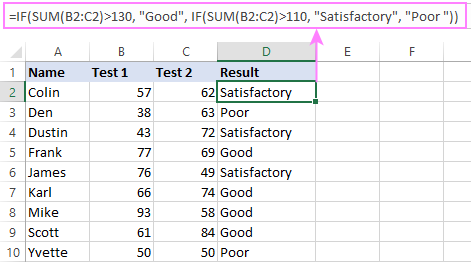
In some situations, your business logic may require including the SUM function in the logical test of IF. For example, to return different text labels depending on the sum of the values in B2 and C2, the formula is:
=IF(SUM(B2:C2)>130, "Good", IF(SUM(B2:C2)>110, "Satisfactory", "Poor"))
If the sum is greater than 130, the result is "good"; if greater than 110 – "satisfactory', if 110 or lower – "poor".
In a similar fashion, you can embed the AVERAGE function in the logical test of IF and return different labels based on the average score:
=IF(AVERAGE(B2:C2)>65, "Good", IF(AVERAGE(B2:C2)>55, "Satisfactory", "Poor"))
Assuming the total score is in column D, you can identify the highest and lowest values with the help of the MAX and MIN functions:
=IF(D2=MAX($D$2:$D$10), "Best result", "")
=IF(D2=MAX($D$2:$D$10), "Best result", "")
To have both labels in one column, nest the above functions one into another:
=IF(D2=MAX($D$2:$D$10), "Best result", IF(D2=MIN($D$2:$D$10), "Worst result", ""))

Likewise, you can use IF together with your custom functions. For example, you can combine it with GetCellColor or GetCellFontColor to return different results based on a cell color.
In addition, Excel provides a number of functions to calculate data based on conditions. For detailed formula examples, please check out the following tutorials:
Example 3. IF with ISNUMBER, ISTEXT and ISBLANK
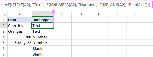
To identify text, numbers and blank cells, Microsoft Excel provides special functions such as ISTEXT, ISNUMBER and ISBLANK. By placing them in the logical tests of three nested IF statements, you can identify all different data types in one go:
=IF(ISTEXT(A2), "Text", IF(ISNUMBER(A2), "Number", IF(ISBLANK(A2), "Blank", "")))
Example 4. IF and CONCATENATE
To output the result of IF and some text into one cell, use the CONCATENATE or CONCAT (in Excel 2016 - 365) and IF functions together. For example:
=CONCATENATE("You performed ", IF(B1>100,"fantastic!", IF(B1>50, "well", "poor")))
=CONCAT("You performed ", IF(B1>100,"fantastic!", IF(B1>50, "well", "poor")))
Looking at the screenshot below, you'll hardly need any explanation of what the formula does:

IF ISERROR / ISNA formula in Excel
The modern versions of Excel have special functions to trap errors and replace them with another calculation or predefined value - IFERROR (in Excel 2007 and later) and IFNA (in Excel 2013 and later). In earlier Excel versions, you can use the IF ISERROR and IF ISNA combinations instead.
The difference is that IFERROR and ISERROR handle all possible Excel errors, including #VALUE!, #N/A, #NAME?, #REF!, #NUM!, #DIV/0!, and #NULL!. While IFNA and ISNA specialize solely in #N/A errors.
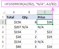
For example, to replace the "divide by zero" error (#DIV/0!) with your custom text, you can use the following formula:
=IF(ISERROR(A2/B2), "N/A", A2/B2)
And that's all I have to say about using the IF function in Excel. I thank you for reading and hope to see you on our blog next week!
Practice workbook for download
Excel IF multiple criteria - examples (.xlsx file)
 by
by
4506 comments
I am trying to write a formula that says: "If the value in I198 is 'ZA' or 'AT', then enter "EIU" in the cell. If I198 is not 'ZA' or 'AT' (if it is any other value) then enter "other".
This is what I have so far, but it's not working.
=IF((OR(I198="ZA", I198="AT")), "EIU", "other")
I have also tried:
=IF(OR(I198="ZA", I198="AT"), "EIU", "other")
Can you help?
HI!
how can I make function SUMS IF instead SUMIFS? :D IF A1=a Than SUM one range, IF A1=b than SUM different range?
thanx
Hi, Dino,
I believe this is what you need for this particular task:
=IF(A1="a",SUM(B:B),IF(A1="b",SUM(C:C),""))
You can add more conditions to sum other ranges by nesting IFs instead of double quotes at the end of the formula.
Hi!
Can someone help me with the below?
I am trying to create a formula in excel to populate the previous columns answers into a points system shown below. The data is being pulled form a research database so the previous column will state the answers show below verbatim. I tried the formula but I keep getting an error. Any advise??
Too High - "I'm a lot worse than I thought" (1 pt)
Too High - "I'm somewhat worse than I thought" (2 pts)
Just Right - "My expectations were met" (3 pts)
Too Low- "I'm somewhat better than I thought" (4 pts)
Too Low- "I'm a lot better than I thought" (5 pts)
=IF(AM4="Too High - "I'm a lot worse than I thought" (1 pt)", "1", IF(AM4="Too High - "I'm somewhat worse than I thought" (2 pts)", "2", IF(AM4="Just Right - "My expectations were met" (3 pts)", "3", IF(AM4="Too Low- "I'm somewhat better than I thought" (4 pts)", "4", IF(AM4="Too Low- "I'm a lot better than I thought" (5 pts)", "5","0")))))
Hi, Chelsea,
you're most likely getting an error because of the double quotes between the phrases: Too High – “I’m a lot worse than I thought”
Try replacing them with single quotes or delete them completely, so that Excel could treat your text values in a proper way.
I made this formula to track the progress of classes based on their start and end dates to Upcoming, Inporgress, and Closed, But this formula is not working properly. Column E is start dates, Column F is the end date.
=IF(AND(E2=TODAY()),"InProgress",IF(AND(F2>TODAY(),E2TODAY(),F2>=TODAY()),"Upcoming","")))
Thanks,
Sarah
A1 = Today/tomorrow
B1 = Profit/Loss
C1 = Numeric Value
Formula Required in D1:
if A1 is today and B1 is profit then 0, but A1 is today but B1 loss then c1*0.025%, but if A1 is tomorrow then c1*0.1%
Means, if A1 is tomorrow then B1 value doeant matter( both prit or loss will give 10%)
I want add number of classes to each subject so that whose attendance percentage is less than 85%. Total number of classes(example 40 classes) which to be added is distributed to each class in such a way that number of attended classes should not more than classes held.
HI ALL,
can u help me with this?
if (A1>=98%, "3", if(A1>=96% but <98%,"2")
if he product category have to deiced where it belongs to and the dimension is given
length width height
9.199 7.199 0.599
and condition is below
(PKG_HEIGHT)<=8.5
(PKG_LENGTH)<=17
(PKG_WIDTH) <=10
then it will belongs to "L"
2nd condition
(PKG_HEIGHT)<=5
(PKG_LENGTH)<= 15
(PKG_WIDTH) <=6.5
them it will belongs to "M"
3rd condition
AND (PKG_HEIGHT)<=5
(PKG_LENGTH)<= 8
(PKG_WIDTH) <=6.5
then it will belongs to "S"
these condition must belongs to dimension , pls help with the formula
Hi there,
I'm hoping you might be able to help if it's not too much trouble.
Based on the format of the formula in this thread, I've built this formula:
=IF((AND(ISBLANK C4, B4=B3)),C3,"")
but this returns a result of #NAME?.
Can you tell me what is wrong?
Basically, I want the formula to first establish that C4 is empty AND that the value in B4 is the same as the value inB3 and then if that is all true, put the value from C3 into the formula field.
I am wanting to populate gaps in 2 columns of numbers that have correlating values that need filling in to the second column in some places but not all.
Example data:
Row2 (A)Image IRN (B)Object Reg (C)Object IRN
Row3 12345 555 ObjectIRN01
Row4 412458 555
Row5 36598 555
Row6 12478 222 ObjectIRN02
Row7 13697 222
So, for example, I would want the value "ObjectIRN01" to be displayed if C4 is blank.
Are you able to assist?
Any help greatly appreciated!
Karen
Hi again, note that I put together an IF AND statement that runs without error.......
=IF((AND(ISBLANK(BLANK C4),B4=B3)),C3,"no match")
...however, in the case where B4 does equal B3, where it should place the value from C3 into the cell where the formula is, it says "no match".
Just in case this helps anyone else, I have since built a list of the reference values and then used an INDEX formula to populate the blank column as required... works like a dream!
Karen
how do i create this formula? I want B17 to show as follows
=if B17 is BASIC should show $0.00 but if PREMIERE should show $85.00 how to create this?
Hi!
Here's the formula:
=IF(B17="BASIC", 0, IF(B17="PREMIERE", 85, ""))
Just enter the formula in a cell, and then apply the currency format to that cell (the fastest way is to press the Ctrl+Shift+$ shortcut).
Hello,
I want to sum the values in Column E but i have a condition that if value in the corresponding Column C=10 then it should take the value from column G instead of Column E.
I used this formula , please suggest a smaller one.
SUM(IF(C2=10,G2,E2),IF(C3=10,G3,E3),IF(C4=10,G4,E4),IF(C5=10,G5,E5),IF(C6=10,G6,E6),IF(C7=10,G7,E7),IF(C8=10,G8,E8),IF(C9=10,G9,E9),IF(C10=10,G10,E10),IF(C11=10,G11,E11),IF(C12=10,G12,E12),IF(C13=10,G13,E13),IF(C14=10,G14,E14))
Hi,
Excel formula for If cell A1 value 1 and B2 value 2, I need total value not more than 2
value value Total Value Not more than
1 2 2
Pls help me
hi there
i have a problem in excell sheet.
a sheet for ATTENDANCE
Hi, I am trying to create a formula for the Following situation:
For Cell E9:
-If the # in E7 is equal to a number in A 2-20, print the corresponding percent to that number from B 2-20 in cell E9.
Example:
A B ..................E
1 12%
2 15%
3 19% (E7): 2
4 23% (E9): 15%
I know this isnt the most clear way of writing this question, but its the best I have with my limited excel knowledge at this time. Any Help is much Appreciated. Thanks!
Hi, Austin,
try the folowing in E9:
=VLOOKUP(E7,A1:B4,2)
(Make sure, to make E9 to indicate percentage. It can be set up under Home tab, Number group).
You can also learn how VLOOKUP works here.
I need a formula that if D4>=10 and F4=yes then "MDR"
I am not sure how to write this.
Thanks,
Sandra
Hello, Sandra,
use IF & AND function so that two conditions are met in order to return 'MDR'. Try this formula:
=IF(AND(D4>=10,F4="yes"),"MDR","")
Hi,
I am trying to put value from the different multiple criteria. But am unable to put IF function. please let me know what's the accurate function for this one
"CLASS/
RELATION" EMPLOYEE SPOUSE CHILD
VIP CLASS 4213 5335 4213
CLASS A 2649 5005 2649
SILVER A 2010 4132 2010
STAFF A 1145 2446 1145
STAFF B 812 1818 812
Hi,
I am trying to figure out how to determine if a date in column G falls with the range of date in column D (greater than) and column F (less than). If it does, then column H should state $110? Sorry I tried to attach the sheet here but didn't work. Please let me know.
Hi,
For that particular case the formula will be:
=IF(AND(G2>D2,G2<F2),110,"")
If it doesn't help, you can send us your worksheet with the data and the result you expect to get to support@ablebits.com. Don't forget to mention your comment and this article.
How can I get the brand name of this item? Who can help me with my problem? TIA
B JORDAN M SIZE 43 BUR 52 - E
ADIDAS M SIZE 42 DE101 5 52
LACOSTE F SIZE 36 842 C90 52
G VANS M SIZE 38 857 C10 55
Please, specify your task: what brand name (you have a list of 4), what do you want to do with it (them) exactly – to return the value into another cell or something else? Give us more details about your task so we could help you.
Hello Natalia,
This is the example of my work, how can I get the brand of my item in column b using formula? Thanks
Example:
Column A Column B
B JORDAN M SIZE 43 BUR 52 - E JORDAN
ADIDAS M SIZE 42 DE101 5 52 ADIDAS
LACOSTE F SIZE 36 842 C90 52 LACOSTE
G VANS M SIZE 38 857 C10 55 VANS
Column A ||| Column B
B JORDAN M SIZE 43 BUR 52 - E ||| JORDAN
ADIDAS M SIZE 42 DE101 5 52 ||| ADIDAS
LACOSTE F SIZE 36 842 C90 52 ||| LACOSTE
G VANS M SIZE 38 857 C10 55 ||| VANS
I need a formula for follwoing
if cell A1:A5 = "A" divide some number by 5
if cell A1:A4 = "A" and A5 does not have any entry then divide some number by 4 .
If your number to divide is in column B, and you want to check whether there's 'A' in every A-cell, then try this formula:
=IF(AND(A1="A", A2="A", A3="A", A4="A"),IF(A5="A",B1/5,IF(A5=" ",B1/4,"")),"")
I want make condition by using IF by which status of particular column could change Like building construction work i enter site drawing date in A column then status in S column should "Site Drawing Completed", then i enter date of work start in B column then status in S column should be "Work Started". How can i do it.
Hello.
can someone, please, help me?
I have a column A and a column B.
In column B I can have up to 99 values (text values/words/phrases) and I want in column A to result another specific value, depending of what value is written in column B.
For example, in column B I have: red, green, white, yellow, black etc.
And in column A i would like to obtain: Aple if column B is red, green or white or.... so on, Mango if column B is green, black, yellow or....so on, and Banana if column B is purple, blue, orange or... so on.
Is there any formula that can help me?
Thank you!
Hello, Sasha,
in your case IF function would be too long and complex.
What may help you better is a VLOOKUP function. It helps to find and return the data inside a large table. But for that you may need to create an additional small table (you can do this on the same sheet) with corresponding matches, like:
red - apple
orange - mango
yellow - banana
white - coconut
and so on
Then try to apply VLOOKUP function.
How can I make excel leave cells blank if a cell in a calculation is blank. I used to use =if(A1,"","")(a1+b2)
Hello John,
Try this one: =IF(A1="","", A1+B2)
Hello! I need help with this formula
=IF(F10:F21="1T", H10:H21,0) it says #VALUE!
What I want to happen is that if in a cell of the column F there is a 1T only then take the value of same cell but in the column H and accumulate it.
Please help me!!!
Hi,sveltana,
i need you help, i am trying to put one formula by using nested loop.
my query is i have different states in my country, where professional tax is different for each state and with different salaries slab.
Ex:-
state 1
slabs rates
upto 15000-nil
15001 to 20000-150
above 20000-200
state 2
slab rates
upto 10000-nil
10001 to 15000-175
15001 to 20000-200
state-3
upto 7500-nil
7501 to 10000-75
10001 to 15000-150
15001 to 20000-200
which is best formula please explain with example.
Hi all,
good day! Can someone help me creating a formula for this? if the Net results fall in any of this category. then fee should be calculated as Net Results*%. for example NET Results is 10001= then Fee=1001*3%
0-500= 1%
501-1000=2%
1001-1500=3%
1501-2000=4%
2001 and above is 5%
Thank you very much for your help.
Check cell 1, whether it contains value R or L, if it contains R check cell 2 whether it contains C or not, if value is C, then check cell 3 and verify that if it contain anyone of V, X,Y & Z, if V display 100, if X means display 101, if Y means display 102 and if Z means display 103
In case if the cell 1 contains L means, then check cell 2 whether it contains C or not, if value is C, then check cell 3 and verify that if it contain anyone of V, X,Y & Z if V display 200, if X means display 201, if Y means display 202 and if Z means display 203
I need to calculate some incentives as below tier:
>=10 pcs sold, incentive $0.20 per pc
>=20 pcs sold, incentive $0.50 per pc
>=30 pcs sold, incentive $0.80 per pc
eg. if the sales staff sold 28 pcs of the item, he will get $0.50 x 28 pcs = $14
How to set formula (using 'IF')?
Hello, Kim
assuming that the number of sold pieces is in A1, the formula will look like this:
=IF(AND(A1>=10,A1<20),A1*0.2,IF(AND(A1>=20,A1<30),A1*0.5,IF(A1>=30,A1*0.8,"")))
Note, that it doesn’t include the numbers that are less than 10, but the result returned for them can be set instead of two quotes at the end of the formula.
To learn more about the function, feel free to read the info on how to create nested IF function together with AND function inside it.
hi again, according to above mentioned comment, i can do this easily with 2 different tables, one of with "W" and "R" and others with "0" and "1" by using =IF(C7="Р",0,1) on the 2nd table with "0" and "1" than using "SUM"
Hi guys,
My question is:
Is is possible to make an schedule by making table, for exmaple:
I have workgroup of 15 people and only 11 must be on daily work, so 4 people must rest per day.
I wanna make a mix formula and my idea is to be like that:
"W" = work
"R" = Rest.
So for "w" should be "0" and for "R" must be "1" , then i can easily calculate how many of them will rest without counting it manually,because the formula will calculate it.
It must be with =SUM(IF(U6:U20="W",0,1))
http://imgur.com/a/MRXI4 a quick example just with "0" and "1" i just do not know how to make the formula, if on the cell is "W" must be understand as "0" and vice verse
Hey, Alex,
there's another simpler function you can use, whether you have numbers in cells
=COUNTIF(U6:U20,0)
or letters
=COUNTIF(U6:U20,"W")
It returns the number of those "Ws" you are trying to sum up.
Read here to find out more about the function.
My question is around the "then" part of the logical test. I want to say "if someone has selected "no" from the picklist, then put "X", if someone has selected "yes" then insert picklist" (with the second picklist being a new one.
E.g. Is it under contract? (dropdown picklist "yes/no". If "yes" is selected, then you need to make a selection in the next column from a dropdown list "Company/Landlord/Dual"
Is this at all possible?
Hello, Tania,
yes, it is somewhat possible. For that you need to create a dependent drop-down list, but your "X" will have to be a part of another drop-down list (it can even be a single choosing option). Using your data, try to follow the steps described in the article.
However, if you want "X" to appear as a simple text without any drop-down lists, you need a special custom script; and, unfortunately, we won't be able to help with it.
I am a manager and have to work with a scheduling program that lists the employees days as such. 08:00P-04:00A 10:00P-06:00A. If the employee works 10:00P-06:00A on Monday and then works 08:00P-04:00A on Tuesday then the company will incur 2 hours of overtime because the employee has not had 16 hours off between shifts. I am looking for a formula that will compare the whole week and let me know where the overlap occurs. There are hundreds of employees and this is a very tedious operation I am hoping to make simple.
Thanks in Advance for the help
i am a dealer..
i sell cars on installments
i need a formula in excel which automatically due the amount after due date.
3 years installment
first installment: 49000
2nd installment: 50000
3rd installment: 50000
every month installment: 8000
33 months installment plan
half year installment: 45000
last installment 66000
I have cell 1 "2.5" i need "2.5"
If cell 1 has "4-6", i need only "6"
,cell 1 has "0.5" i need only "0.5"
if cell 1 has ".25" i need only "1.25"
if cell 1 has 5-4 i need only "4"
if cell 1 has 4-6 i need only "6"
if cell 1 has 6-9 i need only "9"
if cell has 9-14 i need only "14"
is there any formula to extract exact value in on refer cell
Hi,
I want to write a formula for this,
If employee grade is L1 or L2, then date of exit= date of resignation+30days, in case employee grade is L3,L4 OR L5, then then date of exit= date of resignation+60days & in case employee grade is L6 or L7, then date of exit= date of resignation+120 days
kindly help
Hi
I want the result in one cell, like
A1>=B1 then"OK,
C1>=D1 then "OK",
E1>=F1 then "OK"
B1= Blank then "Pending",
D1=Blank then "Pending"
other wise "Not OK.
All this function result in one Cell, Example in G1,
Can this possible. Pls help
Hi, I'm working on a spreadsheet involving dates and I'm unsure which formula to use.
Basically, I want to be able to change the value appearing a cell based on a date range, example:
If after 02/01/2017, I want the cell to read 7
If after 14/04/2017, I want the cell to read 6
If after 17/04/2017, I want the cell to read 5 etc etc.
Is there a suitable formula that I could use?
Thank you.
Can you
Hi, Lucy,
we will be able to assist you better if you send us a sample workbook with your data and the result you want to get to support@ablebits.com. Also, provide a link to this article and your comment. We will take a look at the data and will get back in touch. Thanks!
Dear Sir,
i want pt calculation Formula in excel with three conditions
1- Below 15000-0/-
2-15000 to 1999- Rs.150/-
3-Above 20000 Rs,200/-,
please tell me if formula with three conditions
Can i ask what formula can i use to count for example: i want to count specific name in a column range a2:a5 only if column range b2:b5 has numbers. For example b2=12 and a2=mark, then it is counted. Another if b3 is blank and a3=mark then mark is not counted. So in range a2:a5 has 1 mark name only... sorry if it is confusing.
Hello, Cess,
try this formula:
=COUNTIFS($A$2:$A$5,"mark",B2:B5,">0")
Hope this is what you need.
totally lost on what kinda of function i need here.
A B C
1 Listing X 2%
2 Selling X 3%
3 Formula needed: if B1&2 are both X, then C1+C2 (5%) -or-
if only B1 is X, then C1
if only B2 is X, then C2
Hi,
So I have an issue here is the situation:
Sheet 1
A 1 2 3
A 4 5 6
B 7 8 9
B 10 11 12
And what I need to do is a IF statement where Colomn A (with a A value in the cell) with copy all the cells in that row and insert them into sperate cells on a seperate sheet like this:
Sheet 1 Sheet 2
A 1 2 3 A 1 2 3
A 4 5 6 ---> A 4 5 6
B 7 8 9
B 10 11 12
If you could figure something out it would help me alot. Thanks!!!
Hi Svetlana,
Your help please to do create the formula for below logical test:
if a cell(A) contains urgent request and its aging in another cell(B) is 2, Offtrack
Thank you!
HI I NEED HELP FOR FORMULA TO BE USED IN FOLLOWING CONDITIONS
hi i need formula for following:
A2=783P,A3=782P,C10=782P,C11=990,C12=1348,C13=(=C12)FORMULA,C14=(=C11-48)FORMULA,D10=783P,D11=2121,D12=1290,D13=(=D12)FORMULA,D14=(=D11-48)FORMULA.
REQUIRED FORMULA:IF A2 MATCH WITH C10,RETRIEVE C13:C14 ALONG WITH ITS BUILTUP FORMULA TO C18:C19, IF A2 MATCH WITH D10,RETRIVE D13:D14 ALONG WITH ITS BUILTUP FORMULA TO C18:C19
I want to add a new row when using an IF formula. So IF one cell has a date when the item was returned then add a new row below it with the same asset number from the same item that was returned.
So if A1 with asset number 123 has been returned and cell A8=Returned then insert a new row below it with the same asset number in B1.
Thanks
Hi
I am using an IF statement plus VLOOKUP statement to identify if IDs are the same on both tabs, then determine if certain data in both tabs are the same or different . If it's different it returns REVIEW, if it is the same it returns OK. The problem I'm having is it is not identifying if tab 2 ID is not on tab 1, then return NA or some other text I choose. Here is my current formula. I do not know how to build this into my current formula
=IF(VLOOKUP(FEB2317File!A2,FEB2317File!$A$2:$K$1725,11,0)=MAR2317File!K:K,"ok","REVIEW")
Please help me out with this, in the given table I want to apply conditional formatting based on following procedure:
1st - Get the day based on date
2nd - Then compare the value entered in particular cell, say D2, with respective quota for the day(Mon, Tue, Wed, Thur - Weekdays and Fri, Sat, Sun - Weekends) assigned to the person
3rd - If he exceeds quota then cell colour to be changed to "red"
Table link - https://docs.google.com/spreadsheets/d/1CWm3vdxvMIoxoq0ZlA3Y9M5_tXEtuWKm-iP0RR7pEQ0/edit?usp=sharing
Hello,
Please help me out with this, in the given table I want to apply conditional formatting based on following procedure:
1st - Get the day based on date
2nd - Then compare the value entered in particular cell, say D2, with respective quota for the day(Mon, Tue, Wed, Thur - Weekdays and Fri, Sat, Sun - Weekends) assigned to the person
3rd - If he exceeds quota then cell colour to be changed to "red"
A B C D E
Person Quota Weekdays Quota weekends 01-03-2017 02-03-2017
Hari 1 3
Pari 2 4
Kari 4 4
I have a question, please.
I have a collum with 200 rows, I want to find the average number between that collum. My problem is that between those numbers I have number 0 which I do not want to be taken into consideration when calculating the average. What is the formula for that please?
I WANT TO MANAGE SERIAL NUMBER LIKE
IF I GIVE 123 TO SEVETLANA AND WHEN I ENTER IN CONSUME SEVATLANA AND SERIAL 123 TO ANOTHER SHEET THAN ITS FILL WITH GREEN COLOR IF SERIAL NUMBER IS SAME WHICH I GIVE
OUTWARD CONSUME
A B C D
SEVETLANA 123 SEVETLANA 123(FILL GREEN)
SEVETLANA 124(FILL RED)
HUZEFA 123(FILL RED)
I need a formula that checks if the value of a cell is between 5 and 10 then bring the value 100, if the value of the same cell is between 10 and 15 then bring the value 200 and if the value of the same cell is between 15 and 50 then bring the value 300