The tutorial shows how to create multiple IF statements in Excel with AND as well as OR logic. Also, you will learn how to use IF together with other Excel functions.
In the first part of our Excel IF tutorial, we looked at how to construct a simple IF statement with one condition for text, numbers, dates, blanks and non-blanks. For powerful data analysis, however, you may often need to evaluate multiple conditions at a time. The below formula examples will show you the most effective ways to do this.
How to use IF function with multiple conditions
In essence, there are two types of the IF formula with multiple criteria based on the AND / OR logic. Consequently, in the logical test of your IF formula, you should use one of these functions:
- AND function - returns TRUE if all the conditions are met; FALSE otherwise.
- OR function - returns TRUE if any single condition is met; FALSE otherwise.
To better illustrate the point, let's investigate some real-life formulas examples.
Excel IF statement with multiple conditions (AND logic)
The generic formula of Excel IF with two or more conditions is this:
Translated into a human language, the formula says: If condition 1 is true AND condition 2 is true, return value_if_true; else return value_if_false.
Suppose you have a table listing the scores of two tests in columns B and C. To pass the final exam, a student must have both scores greater than 50.
For the logical test, you use the following AND statement: AND(B2>50, C2>50)
If both conditions are true, the formula will return "Pass"; if any condition is false - "Fail".
=IF(AND(B2>50, B2>50), "Pass", "Fail")
Easy, isn't it? The screenshot below proves that our Excel IF /AND formula works right:

In a similar manner, you can use the Excel IF function with multiple text conditions.
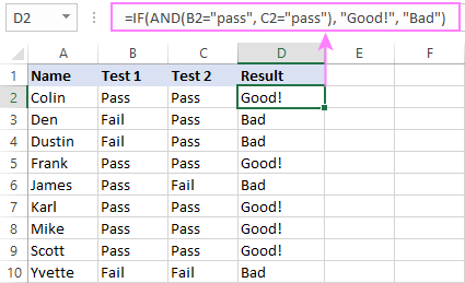
For instance, to output "Good" if both B2 and C2 are greater than 50, "Bad" otherwise, the formula is:
=IF(AND(B2="pass", C2="pass"), "Good!", "Bad")
Important note! The AND function checks all the conditions, even if the already tested one(s) evaluated to FALSE. Such behavior is a bit unusual since in most of programming languages, subsequent conditions are not tested if any of the previous tests has returned FALSE.
In practice, a seemingly correct IF statement may result in an error because of this specificity. For example, the below formula would return #DIV/0! ("divide by zero" error) if cell A2 is equal to 0:
=IF(AND(A2<>0, (1/A2)>0.5),"Good", "Bad")
The avoid this, you should use a nested IF function:
=IF(A2<>0, IF((1/A2)>0.5, "Good", "Bad"), "Bad")
For more information, please see IF AND formula in Excel.
Excel IF function with multiple conditions (OR logic)
To do one thing if any condition is met, otherwise do something else, use this combination of the IF and OR functions:
The difference from the IF / AND formula discussed above is that Excel returns TRUE if any of the specified conditions is true.
So, if in the previous formula, we use OR instead of AND:
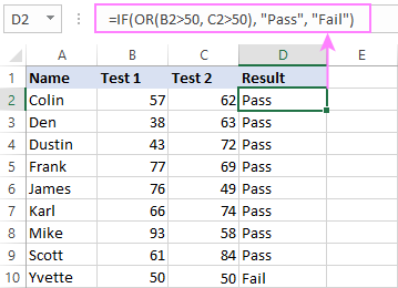
=IF(OR(B2>50, B2>50), "Pass", "Fail")
Then anyone who has more than 50 points in either exam will get "Pass" in column D. With such conditions, our students have a better chance to pass the final exam (Yvette being particularly unlucky failing by just 1 point :)
Tip. In case you are creating a multiple IF statement with text and testing a value in one cell with the OR logic (i.e. a cell can be "this" or "that"), then you can build a more compact formula using an array constant.
For example, to mark a sale as "closed" if cell B2 is either "delivered" or "paid", the formula is:
=IF(OR(B2={"delivered", "paid"}), "Closed", "")
More formula examples can be found in Excel IF OR function.
IF with multiple AND & OR statements
If your task requires evaluating several sets of multiple conditions, you will have to utilize both AND & OR functions at a time.
In our sample table, suppose you have the following criteria for checking the exam results:
- Condition 1: exam1>50 and exam2>50
- Condition 2: exam1>40 and exam2>60
If either of the conditions is met, the final exam is deemed passed.
At first sight, the formula seems a little tricky, but in fact it is not! You just express each of the above conditions as an AND statement and nest them in the OR function (since it's not necessary to meet both conditions, either will suffice):
OR(AND(B2>50, C2>50), AND(B2>40, C2>60)
Then, use the OR function for the logical test of IF and supply the desired value_if_true and value_if_false values. As the result, you get the following IF formula with multiple AND / OR conditions:
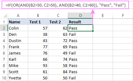
=IF(OR(AND(B2>50, C2>50), AND(B2>40, C2>60), "Pass", "Fail")
The screenshot below indicates that we've done the formula right:
Naturally, you are not limited to using only two AND/OR functions in your IF formulas. You can use as many of them as your business logic requires, provided that:
- In Excel 2007 and higher, you have no more than 255 arguments, and the total length of the IF formula does not exceed 8,192 characters.
- In Excel 2003 and lower, there are no more than 30 arguments, and the total length of your IF formula does not exceed 1,024 characters.
Nested IF statement to check multiple logical tests
If you want to evaluate multiple logical tests within a single formula, then you can nest several functions one into another. Such functions are called nested IF functions. They prove particularly useful when you wish to return different values depending on the logical tests' results.
Here's a typical example: suppose you want to qualify the students' achievements as "Good", "Satisfactory" and "Poor" based on the following scores:
- Good: 60 or more (>=60)
- Satisfactory: between 40 and 60 (>40 and <60)
- Poor: 40 or less (<=40)
Before writing a formula, consider the order of functions you are going to nest. Excel will evaluate the logical tests in the order they appear in the formula. Once a condition evaluates to TRUE, the subsequent conditions are not tested, meaning the formula stops after the first TRUE result.
In our case, the functions are arranged from largest to smallest:
=IF(B2>=60, "Good", IF(B2>40, "Satisfactory", "Poor"))
Naturally, you can nest more functions if needed (up to 64 in modern versions).

For more information, please see How to use multiple nested IF statements in Excel.
Excel IF array formula with multiple conditions
Another way to get an Excel IF to test multiple conditions is by using an array formula.
To evaluate conditions with the AND logic, use the asterisk:
To test conditions with the OR logic, use the plus sign:
To complete an array formula correctly, press the Ctrl + Shift + Enter keys together. In Excel 365 and Excel 2021, this also works as a regular formula due to support for dynamic arrays.
For example, to get "Pass" if both B2 and C2 are greater than 50, the formula is:
=IF((B2>50) * (C2>50), "Pass", "Fail")

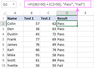
In my Excel 365, a normal formula works just fine (as you can see in the screenshots above). In Excel 2019 and lower, remember to make it an array formula by using the Ctrl + Shift + Enter shortcut.
To evaluate multiple conditions with the OR logic, the formula is:
=IF((B2>50) + (C2>50), "Pass", "Fail")
Using IF together with other functions
This section explains how to use IF in combination with other Excel functions and what benefits this gives to you.
Example 1. If #N/A error in VLOOKUP
When VLOOKUP or other lookup function cannot find something, it returns a #N/A error. To make your tables look nicer, you can return zero, blank, or specific text if #N/A. For this, use this generic formula:
For example:
If #N/A return 0:
If the lookup value in E1 is not found, the formula returns zero.
=IF(ISNA(VLOOKUP(E1, A2:B10, 2,FALSE )), 0, VLOOKUP(E1, A2:B10, 2, FALSE))
If #N/A return blank:
If the lookup value is not found, the formula returns nothing (an empty string).
=IF(ISNA(VLOOKUP(E1, A2:B10, 2,FALSE )), "", VLOOKUP(E1, A2:B10, 2, FALSE))
If #N/A return certain text:
If the lookup value is not found, the formula returns specific text.
=IF(ISNA(VLOOKUP(E1, A2:B10, 2,FALSE )), "Not found", VLOOKUP(E1, A2:B10, 2, FALSE))

For more formula examples, please see VLOOKUP with IF statement in Excel.
Example 2. IF with SUM, AVERAGE, MIN and MAX functions
To sum cell values based on certain criteria, Excel provides the SUMIF and SUMIFS functions.
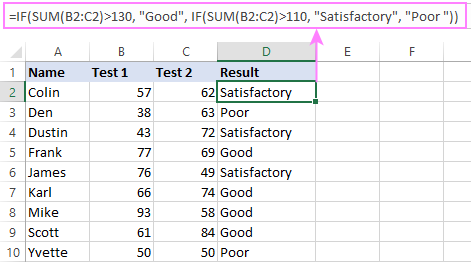
In some situations, your business logic may require including the SUM function in the logical test of IF. For example, to return different text labels depending on the sum of the values in B2 and C2, the formula is:
=IF(SUM(B2:C2)>130, "Good", IF(SUM(B2:C2)>110, "Satisfactory", "Poor"))
If the sum is greater than 130, the result is "good"; if greater than 110 – "satisfactory', if 110 or lower – "poor".
In a similar fashion, you can embed the AVERAGE function in the logical test of IF and return different labels based on the average score:
=IF(AVERAGE(B2:C2)>65, "Good", IF(AVERAGE(B2:C2)>55, "Satisfactory", "Poor"))
Assuming the total score is in column D, you can identify the highest and lowest values with the help of the MAX and MIN functions:
=IF(D2=MAX($D$2:$D$10), "Best result", "")
=IF(D2=MAX($D$2:$D$10), "Best result", "")
To have both labels in one column, nest the above functions one into another:
=IF(D2=MAX($D$2:$D$10), "Best result", IF(D2=MIN($D$2:$D$10), "Worst result", ""))

Likewise, you can use IF together with your custom functions. For example, you can combine it with GetCellColor or GetCellFontColor to return different results based on a cell color.
In addition, Excel provides a number of functions to calculate data based on conditions. For detailed formula examples, please check out the following tutorials:
Example 3. IF with ISNUMBER, ISTEXT and ISBLANK
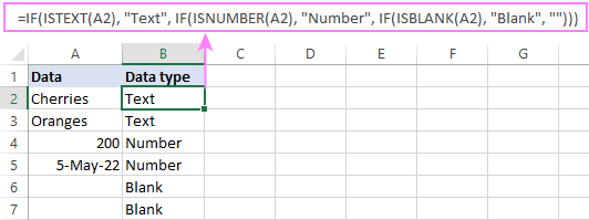
To identify text, numbers and blank cells, Microsoft Excel provides special functions such as ISTEXT, ISNUMBER and ISBLANK. By placing them in the logical tests of three nested IF statements, you can identify all different data types in one go:
=IF(ISTEXT(A2), "Text", IF(ISNUMBER(A2), "Number", IF(ISBLANK(A2), "Blank", "")))
Example 4. IF and CONCATENATE
To output the result of IF and some text into one cell, use the CONCATENATE or CONCAT (in Excel 2016 - 365) and IF functions together. For example:
=CONCATENATE("You performed ", IF(B1>100,"fantastic!", IF(B1>50, "well", "poor")))
=CONCAT("You performed ", IF(B1>100,"fantastic!", IF(B1>50, "well", "poor")))
Looking at the screenshot below, you'll hardly need any explanation of what the formula does:

IF ISERROR / ISNA formula in Excel
The modern versions of Excel have special functions to trap errors and replace them with another calculation or predefined value - IFERROR (in Excel 2007 and later) and IFNA (in Excel 2013 and later). In earlier Excel versions, you can use the IF ISERROR and IF ISNA combinations instead.
The difference is that IFERROR and ISERROR handle all possible Excel errors, including #VALUE!, #N/A, #NAME?, #REF!, #NUM!, #DIV/0!, and #NULL!. While IFNA and ISNA specialize solely in #N/A errors.
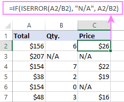
For example, to replace the "divide by zero" error (#DIV/0!) with your custom text, you can use the following formula:
=IF(ISERROR(A2/B2), "N/A", A2/B2)
And that's all I have to say about using the IF function in Excel. I thank you for reading and hope to see you on our blog next week!
Practice workbook for download
Excel IF multiple criteria - examples (.xlsx file)
 by
by
4506 comments
Hi, I want a formula in F1 to pick up only one result:
If C1>=1 and C2 to C5 = 0, then D1*E1, othewise D1*E2
If C2>=1 and C3 to C5 = 0, then D1*E2, otherwise D1*E3
If C3>=1 and C4 & C5 = 0, then D1*E3, otherwise D1*E4
If C4>=1 and C5 = 0, then D1*E4, otherwise D1*E5
If C5>=1, then D1*E5
Is it possible to set a formula like this?
Many thanks
Hi, hopefully, you can help. I have 2 columns of data. In the first column is Male (M) and Female (F). The second column has their score totals.
I would like the TOP 3 males to be highlighted Green and top three females highlighted Yellow. Is this possible?
Good day
please assist with the following senario, please ignore my prev post
=IF(AND([@AbcClass]>=$A$1,[@AbcClass]=$A$2,[@AbcClass]<$A$3),[@[12 mnt AveQtysold ]]*"2")and so worth, but it comes up with an error
regards
Cindy
good day
please assist with the following senario
=IF(AND([@AbcClass]>=$A$1,[@AbcClass]=$A$2,[@AbcClass]<$A$3),[@[12 mnt AveQtysold ]]*"2")and so worth, but it comes up with an error
regards
Cindy
The three above make one line I put in the cell. There should be a 0 after the I2>
Whew!!
Hi Maria,
First off, our apologies for mangled formulas. Our blog engine has problems with posting formulas containing < and > signs.
In case of nested IF's, the conditions are checked in the order they appear in the formula, and if the first condition is TRUE, others are not checked. So, you simply put the I2>0 statement first, like this:
=IF(I2>0, "Completed", IF(E2<0, "Expired", IF(E2<10, "Expiring soon", "")))
IF(I2>),"Completed","")))
IF(E2<10,"Expiring soon",
Really!!
IF(E2<0,"Expired",
Darn it! It won't let me copy and paste it correctly.
+IF(E2<0,"Expired",IF(E20,"Completed","")))
Sorry wrong formula above. This is the right one.
=IF(E2<0,"Expired",IF(E20,"Completed","")))
Hi. I'm trying to use the =IF formula to calculate based on dates if a cell will show "Expired", "Expiring soon", or "Completed. It looks like this-
=IF(E2<0,"Expired",IF(E20,"Completed",""))).
In column E is a number for how many days a letter needs to be mailed out (30, 60, 90, etc). This part works and shows "Expired" if the due date has passed and it's to late to send a letter, and "Expiring soon" if it is 10 days or less until the due date. I made a column I to put in a date that the letter was sent. I have several rows that display "Expiring soon", but when I put a date that I sent the letter to show that it's been completed and mailed out, the "Expiring soon" won't change to "Completed". I'd really appreciate it if you can help me fix this. Thank you.
looking for a solution to this IF formula issue.
IF Reqd By Date Reqd By Date = "FAIL"
if it is complete before RBD? y= PASS N=FAIL
if it isn't complete is it before the required by date? y= PASS N=FAIL
if it is not complete and > than the Reqd By Date =FAIL
Sorry formula pasted wrongly, Below is the which I wrote
=IF(AND(D1='Billing Calander'!$C$3),"Jan'16","")
I tried the below formula for 1 condition but not working
=IF(AND(D1='Billing Calandar'!$C$1),"Jan'16","")
billing calandar is nothing but I pasted the criteria in another sheet name as billing sheet.
Pls help me
Hi,
I need the formula for the below condition.
I have the dates in 1 column, Like below
Invoice Date
28-Nov-16
30-Nov-16
1-Dec-16
23-Dec-16
26-Dec-16
28-Dec-16
30-Dec-16
31-Dec-16
1-Jan-17
23-Jan-17
19-Jan-17
if the above column cell date comes between the below criteria like start date & end date it should reflect as Nov'16,Dec'16, Jan'17, Feb'17 etc
Month Start Date End Date
Jan'16 28-Dec-15 22-Jan-16
Feb'16 25-Jan-16 26-Feb-16
Mar'16 29-Feb-16 25-Mar-16
Apr'16 28-Mar-16 22-Apr-16
May'16 25-Apr-16 27-May-16
Jun'16 30-May-16 24-Jun-16
Jul'16 27-Jun-16 22-Jul-16
Aug'16 25-Jul-16 26-Aug-16
Sep'16 29-Aug-16 23-Sep-16
Oct'16 26-Sep-16 21-Oct-16
Nov'16 24-Oct-16 25-Nov-16
Dec'16 28-Nov-16 23-Dec-16
If net change>1, Volume>5, OI>3 then result should be BUY,
if net change5, OI>3 then result should be SELL and the rest should be NEUTRAL.
please help me, how to do it in excel using formula.
Hi,
I am trying to figure out how to use the formulas you provided for this situation:
Let's say:
Column H: Cognitive Score
Column K: Manual Score
Column M: Pass/Fail
Here is what I would like:
If Column H AND Column K both have scores above 357, Column M will say PASS.
If Column H AND Column K both have scores below 357, Column M will say FAIL.
If Column H had a score higher than 357 and Column K had a score lower than 357, Column M will say FAIL MANUAL.
If Column H had a score lower than 357 and Column K had a score higher than 357, Column M will say FAIL COGNITIVE.
Example:
Cognitive Manual Pass/Fail
400 560 PASS
200 100 FAIL BOTH
500 200 FAIL MANUAL
315 600 FAIL COGNITIVE
Any help is appreciated!
Thanks.
Here is my dilemma I have two columns, column J has and issued date and if it is greater than 30 days my formula states to "Contact Owner", otherwise leave blank. This works great. However I need a second part so that if column K2 is not blank then the cell with the formula should be blank, because column K is the closed date.
=IF((TODAY()-J2)>30,"Contact Owner","")
Having a problem with if then. For a promotion roster if A1=1 then private, if A1=2 then private first class, if A1=3 then lance corporal.......
Here is current formula
=IF(J2=1,"Private",IF(J2=2,Private First Class,IF(J2=3,Lance Corporal,IF(J2=4, Corporal))))
It will work for the first function (J2=1) but no other.
Thanks
Will
Correction...here is current forumula.
=IF(J2=1,"Private",IF(J2=2,”Private First Class”,IF(J2=3,”Lance Corporal”,IF(J2=4,“Corporal”))))
When I type 1, Private is properly displayed. All other numbers (2, 3, 4) result in a #NAME? error
Solved it. Had to do with improper quotation marks. Not sure how, but they seemed to be facing the wrong way.
Hi Friends, I am happy to see this is great bunch of knowledge group.
Please help me to arrive the late minutes in the below scenario.
In a single formula, need to get the late minutes,
with multiple criteria.
Cri-1
if IN time is greater than the Grace Time,
Permission is zero,
then Late Minute should arrive the deducted minutes.
Cri-2
if Permission is greater than the Grace Time,
exclude the grace time (should not consider),
put ZERO if IN Time is less than the Permission,
Cri-3
if the IN Time is greater than the Permission, then put the deducted minutes.
Shift Time 9:00
IN Time 9:20
Grace Time 0:15
Permission 0:30
Late Minutes
sunita
muta
samir
sanit
count if used of two staring word of this list
Hi all,
i want to compare 4 columns like columns A,B,C,D.If col A matches with col C and col B matches with col D it should highlight in green color.If it is not matches , highlight in red color in a single condition.Can you help me?
hai i am working in excel sheet
i want if condition
in completely "text" basis
not logical
how?
the formula for L currenlty is =IF(J11="",IF(K11>0.15,"Overdue","Open"),IF(K11>0.15,"Closed Late","Closed"))
A
Hi I need help with my formula.
K = start date
H = due date
J = date completed
K = overdue days '=IF(I6="",-100,(IF(NOW()0.15,"Overdue","Open"),IF(K7>0.15,"Closed Late","Closed"))
I want to add to task status that if start day is more than today it must be "in progress" if less than today then "Not Started. but keep the rest that is in J. How do i do it... I have tried but get a value error or the rest does not work
Please help me.
Anne
Apologies lets try this again.... need to keep L status and add "in progress" and "Not Started"
K = start date
H = due date
J = date completed
K = overdue days
L = Task Status
the formal for K is =IF(I7="",-100,(IF(NOW()0.15,"Overdue","Open"),IF(K7>0.15,"Closed Late","Closed"))
I would life to add to L the status "In progress" and "Not Started" thus if H is less or more than today but keep the rest of L
Thanks :-)
Annemarie
Very helpful. Brilliant work. God bless you.
Why was this comment?
I NEED A HELP WITH A CONDITION TO CALCULATE WITH IF FUNCTION.
PLEASE IF ANYONE CAN HELP LET ME KNOW
CONDITION AS BELOW:
WANT TO CALCULATE THE PROGRESSIVE ADDITION OF MINUTES AND SECONDS MANUALLY WHICH HAVE A CUT OFF OF 60. FURTHER NEED THIS CALCULATION TO BE MODIFIED.
FORMULA FOR THE CALCULATION OF PROGRESSIVE ADDITION OF SECONDS IS
=(IF((M12+M13)>=60,(M12+M13)-60,IF((M12+M13)=60,(IF((M12+M13)>59,(L12+L13)-70+1,(L12+L13)-60)),IF((L12+L13)>60,(L12+L13)+1,(L12+L13))))
CRITERIA REQUIRED IS
1. IF ADDITION OF 2 TIMINGS IS GREATER THAN 60 RESULT MUST BE THE DIFFERENCE AFTER DEDUCTING 60
2. IF THE ADDITION IS EQUAL TO 60 RESULT MUST BE 0
3. IF THE ADDITION IS LESS THAN 60 RESULT MUST BE THE ADDITION FIGURE.
4. IF THE ADDITION OF SECONDS EXCEEDS OR IS EQUAL TO 60 THEN 1 MUST BE BORROWED AT MINUTES CALCULATION FOR ADDITION.
FOR ABOVE CONDITIONS IF ANYBODY CAN SUGGEST SOMETHING PLEASE REPLY.
HOPE I GET SOME ASSISTANCE.
Hi,
How can insert symbols in my true or false value
Hi,
How to perform
Cell A> 3 - to apply this formula ( cell B x 4% x 4.5)
Cell A< 3 - to apply this formula ( cell B x 30% x 4% x 4.5)
Hi, Please suggest to count and add Yes in a row and give a value in number to it and get the score. Example : A1:C1 - "Yes" value -6*3 = 18 similarly if (A1,C1,G1,h1, "Yes" value- 5,4,3,5)
How to perform a SUM count of cells already containing formulas in them. Example
Col A Col B Col C
Sum formula Sum Formula Sum(A+B)
Help would be appreciated.
I am having trouble with this formula.
=IF($M4>=$K4,"Yes",IF(AND($M4<$K4,TODAY<=$G4+274),"Pending",IF(AND($M4$G4+274),"No")))
It returns "Yes" as appropriate, but is returning #NAME? when "No" or "Pending" should come back.
I am not sure where I went wrong. Any help would be appreciated. Thanks in advance.
Thank you so much!
It really works!
You save a lot of my tame!
Hi ya
I need a nested IF function for the following.
I need a cell to come back with a yes if a date in another cell is older than 3 years from today and no if it is within the 3 years
Any help with this would be great
Many thanks
Nicky
Hi
I am trying to complete multiple formulas in one cell.
I would like:
In cell L3, If cell G3 has "Green" entered then it gives the date in cell c3+90 days. If cell G3 has "red" entered it gives the date in cell J3+14 days. Is this possible please?
Hi,
I need to get formula for the values above & below 1.5 million and in the same column above & below 5 million.
I made this but not able to get anything for values above or below 5 million.
Could you please help.
G2 is my cell of amount
=IF(G2>=1500000,"Above 15 Lakhs",IF(G2<1500000,"Below 15 Lakhs",IF(G2=5000000,"Above 50 Lakhs"))))
i want a help my doubt is
A1="SC" A6 SHOULD "CT-HDG-SC"
IF A1 ANY VALUE A6 = (A1&B1&C1)
Note : "sc" is only text and "ct-hdg-sc" also text
Hi!
please help me with formula. example:
channel: forwarding agents: Brands:
retail 1 John Nivea,Orimi,schwarzkopf
retail 2 David Orimi,ufood,schwarzkopf
retail 3 Kerry Schwarzkopf,nivea,orimi
i have 12 channels and 7 brands
the formula must divide automatically for example:
John must delivery only channel 1 if it is = nivea or orimi or schwarzkopf AND david must delivery only channel 2 if it is = orimi,ufood,scwarzkopf,
please help me..
I am trying to use the IF AND statement to verify two criteria with another excel sheet in the same workbook. So I have the following statement //
=IF((AND(C$1='Data Entry Form'!$C:$C,'2017'!$A2='Data Entry Form'!$A:$A)),"P"," ") //
Now this returns only the first match on the entry log sheet. The setup is as such.
Sheet 1 - Row 1 are the Dates for 2017 (all dates included)
and in Column A there is a corresponding number.
Sheet 2 (entry logs) - Column A are the same numbers as the sheet 1 Column A numbers (however these are entered in with different Dates in Col C on Sheet 2.)
I am looking for a formula that checks Sheet 1 Col A and Cell C$1 with the entry log's respective columns for any that match that criteria and if true to place "P" in the corresponding box on Sheet 1.
My issue is it is not recognizing another entry with a different date on the entry log.
Please help.
THank you.
I have a range of cells F9:U9 which contains alphabetical and numbers data. What i need is a formula to apply on this range so i can get the following results
If the range contains the word "Cured" - then in cell V9 (status cell) shows "Cured"
If the Range contains the word "Default" then the status cell would show "Defaulter"
and if there is no entry or numerical entry within the range...then the status cell would show "In Program"
Hi, I am trying to do up a pay sheet. I'm sure the answer is simple, but I can't think of it, so would appreciate your help. In row 1 I have Mon through to Sun. In row 2 I have the hours worked each day. The formula needs to show ordinary hours and overtime hours. So, for example, I imagined that using and if function: =if(a2<=8,A2,8,+if(b2<=8,B2,8,+if(B3<=8.... and so on for the week. Obviously the + isn't adding the cells to give me a final result. Can you help please.
Sorry, got it sorted
I have 2 Sheet, in 1st from the list select the financier name & in 2nd sheet financier list available in which defined which are pvt financier, commercial financier & etc. I want to use to identify in first sheet to from the financier name to identify it is pvt financier or commercial etc. A list of financier is approx 100+, so not easily to use or command.
I tried a formula but not correct
=IF(OR([@Bank]=Sheet1!A3:A4),"Cash",IF(OR([@Bank]=Sheet1!A5:A37),"Comm.", IF(OR([@Bank]=Sheet1!A38:A79),"Pvt.",IF(OR([@Bank]=Sheet1!A80:A124),"RRB","TMP"))))
Hello,
I need help with a nested formula for the following condition please.
if A1>=100% and 104.99% it should return 110%
105% up to 109.99% should return 120%
110% up to 119.99% should return 125%
120% and above should return 135%
Thank you!
If E3 is equal to “j” and F3 is not blank move a negative F3 to J3
Else if E3 is equal to “j” and F3 is blank move H3-G3 to J3
Hello
I am very new at creating formula's and am self taught. I have a bookkeeping document that list numbers that has been assigned to person and a dollar amount in the next column. New amounts will be listed on this sheet each week. Each week I would like the amount from each person transferred to another column for each week automatically when an amount is entered next to their number. I am looking to create a formula that will allow me to do the following:
I have a set of numbers from 1-30 in column A (these numbers may not be in order)and a dollar amount in column B. I have a second column (Column H) that has the same numbers 1-30 (The numbers will be in order).
Is there a formula that I can create that would automatically transfer the amount entered in column B for the person in column A to column I based on the number being the same as the number in column A.
A B H I
Member# Amount Member# Amount
30 $25.00 28 $
50 $15.00 30 $(how can I get amount for
35 $40.00 35 $ member#30 to transfer to
28 $40.00 50 $Column I for #30)
Is it possible to create multiple If functions if the first value it text as well?
My current formula is =IF(M2="C", "Conditional", N2) however I was to add additional text values e.g. =IF(M2="I", "Interview", N2)
Thanks
Hi!
Please help. Why do I get a '#VALUE!' error for the formula " =SUM(IF(O11:O1625="",0,1)*IF(Q11:Q1625="",0,1)*IF(O11:O1625>Q11:Q1625,1,0))" . It looks correct...
I currently am using the following formula to average the cells but if ALL of the cells are blank to say BLANK: =IFERROR(AVERAGE(H19:AI19),"BLANK")
but I need to argue that if the text DO is in any of the cells H19:AI19 then say DO
hi, I need a formula for following condition
for specific value e.g
97
100% of 0-30 + 50% of 30-50 + 30% of 50-70 + 20% of 70-100
Hello,
I want a formula for below problem.
Problem:-
If we are dividing a number with the perfect squares(like 2^2,3^2,4^2,5^2.......etc) when this condition is satisfies with the any of these squares then return the result after the division. Elseif return the original number.
Example:-
sqrt(44)/4=2.sqrt(11)(Here 44 is divisible by 4)
sqrt(99)/9=3.sqrt(11)(Here 99 is divisible by 9)
.
.