The tutorial shows how to extract number from various text strings in Excel by using formulas and the Extract tool.
When it comes to extracting part of a text string of a given length, Excel provides three Substring functions (Left, Right and Mid) to quickly handle the task. When it comes to extracting numbers from an alphanumeric string, Microsoft Excel provides… nothing.
To get a number from a string in Excel, it takes a little ingenuity, a bit of patience, and a bunch of different functions nested into each other. Or, you can run the Extract tool and have the job done with a mouse click. Below you will find full details on both methods.
How to extract number from the end of text string
When you have a column of alphanumeric strings where number comes after text, you can use the following formula to get it.
We will dwell on the formula's logic a bit later. For now, simply replace cell with a reference to the cell containing the original string (A2 in our case), and enter the formula in any empty cell in the same row, say in B2:
=RIGHT(A2, LEN(A2) - MAX(IF(ISNUMBER(MID(A2, ROW(INDIRECT("1:"&LEN(A2))), 1) *1)=FALSE, ROW(INDIRECT("1:"&LEN(A2))), 0)))
This formula gets number only from the end. If a string also has numbers in the beginning or middle, they are ignored:
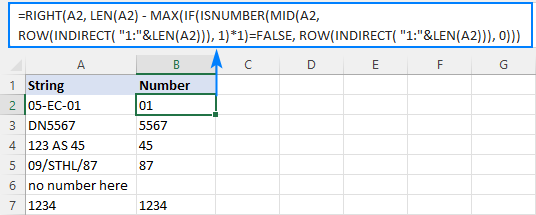
The extraction is performed with the RIGHT function that belongs to the category of Text functions. The output of this function is always text. In our case, the result is a numeric substring, which in terms of Excel is also text, not number.
If you need the result to be a number (that you can use in further calculations), then wrap the formula into the VALUE function or perform an arithmetic operation that does not change the result, say, multiply by 1 or add 0. To catch errors in the strings that do not contain a single number, use the IFERROR function. For example:
=IFERROR(VALUE(RIGHT(A2, LEN(A2) - MAX(IF(ISNUMBER(MID(A2, ROW(INDIRECT("1:"&LEN(A2))), 1)*1)=FALSE, ROW(INDIRECT("1:"&LEN(A2))), 0)))), "")
or
=IFERROR(RIGHT(A2, LEN(A2) - MAX(IF(ISNUMBER(MID(A2, ROW(INDIRECT("1:"&LEN(A2))), 1) *1)=FALSE, ROW(INDIRECT("1:"&LEN(A2))), 0))) +0, "")
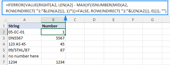
Note. In Dynamic Array Excel (Office 365 and 2021), you enter the formula in the usual way with the Enter key. In Excel 2019 and earlier, it only works as an array formula, so remember to press Ctrl + Shift + Enter to complete it.
How this formula works:
To extract number from an alphanumeric string, the first thing you need to know is where to start the extraction. The position of the last non-numeric character in a string is determined with the help of this tricky formula:
MAX(IF(ISNUMBER(MID(A2, ROW(INDIRECT("1:"&LEN(A2))), 1)*1)=FALSE, ROW(INDIRECT("1:"&LEN(A2))), 0))
To understand the logic, let's investigate it from the inside:
The ROW(INDIRECT("1:"&LEN(A2))) combination creates a sequence of numbers corresponding to the total of characters in the source string (A2), and we serve these sequential numbers to MID as the starting numbers:
MID(A2, {1;2;3;4;5;6;7;8}, 1)
The MID function pulls each individual character from A2 and returns them as an array:
{"0";"5";"-";"E";"C";"-";"0";"1"}
As MID is a text function, its output is always text (as you can notice, all the characters are enclosed in quotation marks). To turn numeric ones into numbers, we multiply the array by 1 (double negation --MID() will have the same effect). The result of this operation is an array of numbers and #VALUE! errors representing non-numeric characters:
ISNUMBER({0;5;#VALUE!;#VALUE!;#VALUE!;#VALUE!;0;1})
The ISNUMBER function evaluates each element of the array and gives its verdict in the form of Boolean values - TRUE for numbers, FALSE for anything else:
{TRUE;TRUE;FALSE;FALSE;FALSE;FALSE;TRUE;TRUE}
This array goes to the logical test of the IF function, where each element of the array is compared against FALSE:
IF({TRUE;TRUE;FALSE;FALSE;FALSE;FALSE;TRUE;TRUE}=FALSE, ROW(INDIRECT("1:"&LEN(A2))), 0)
For each FALSE (non-numeric value), another ROW(INDIRECT()) function returns its relative position in the string. For each TRUE (numeric value), a zero is returned. The resulting array looks as follows:
{0;0;3;4;5;6;0;0}
The rest is easy. The MAX function finds the highest number in the above array, which is the position of the last non-numeric value in the string (6 in our case). Simply, subtract that position from the total length of the string returned by LEN, and pass the result to RIGHT to let it know how many characters to extract from the right side of the string:
RIGHT(A2, LEN(A2) - 6)
Done!
How to extract number from the beginning of text string
If you are working with records where text appears after number, you can extract number from the start of a string by using this generic formula:
With the original string in A2, use the following formula to get number:
=LEFT(A2, MATCH(FALSE, ISNUMBER(MID(A2, ROW(INDIRECT("1:"&LEN(A2)+1)), 1) *1), 0) -1)
No matter how many digits are in the middle or end, only the starting number is extracted:

Note. In Excel 365 and Excel 2021, due to support for dynamic arrays, a regular formula works fine. In Excel 2019 and earlier, you should press Ctrl + Shift + Enter to explicitly make it an array formula.
How this formula works:
Here, we again use the combination of ROW, INDIRECT and LEN functions to create a sequence of numbers equal to the total of characters in the source string plus 1 (the role of that additional character will become clear a bit later).
ROW(INDIRECT("1:"&LEN(A2)+1))
MID and ISNUMBER do the same job as in the previous example - MID pulls individual characters and ISNUMBER converts them to the logical values. The resulting array of TRUE's and FALSE's goes to the MATCH function as a lookup array:
MATCH(FALSE, {TRUE;TRUE;FALSE;FALSE;FALSE;FALSE;TRUE;TRUE;FALSE}, 0)
MATCH computes a relative position of the first FALSE, giving us the position of the first non-numeric character in the string (3 in A2). To extract the preceding numbers, we subtract 1 from position the first text character and serve the difference to the num_chars argument of the LEFT function:
LEFT(A2, 3-1)
Now, back to an "extra" character in the sequence generated by ROW(INDIRECT()+1)). As you already know, this sequence provides the starting points for the MID function. Without +1, MID would extract exactly as many characters as there are in the original string. If the string contains only numbers, ISNUMBER will return only TRUE's while MATCH needs at least one FALSE. To ensure that, we add one more character to the total length of the string, which the MID function would convert to an empty string. For example, in B7, MID returns this array:
{"1";"2";"3";"4";""}
Note. As is the case with the RIGHT function, LEFT also returns a numeric substring, which is technically text, not number. To get the result as a number rather than a numeric string, nest the formula in the VALUE function or multiply the result by 1 as shown in the first example.
How to get number from any position in a string
If your task implies extracting number from anywhere in a string, you can make use of the following mind-boggling formula published on MrExcel forum:
=SUMPRODUCT(MID(0&A2, LARGE(INDEX(ISNUMBER(--MID(A2, ROW(INDIRECT("1:"&LEN(A2))), 1)) * ROW(INDIRECT("1:"&LEN(A2))), 0), ROW(INDIRECT("1:"&LEN(A2))))+1, 1) * 10^ROW(INDIRECT("1:"&LEN(A2)))/10)
Where A2 is the original text string.
Breaking down this formula would require a separate article, so you can simply copy it to your worksheet to make sure it really works :)
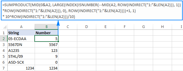
Upon examining the results, however, you may notice one insignificant drawback - if the source string does not contain a number, the formula returns zero, as in row 6 in the screenshot above. To fix this, you can wrap the formula in the IF statement, the logical test of which checks if the source string contains any number. If it does, the formula extracts the number, otherwise returns an empty string:
=IF(SUM(LEN(A2)-LEN(SUBSTITUTE(A2, {"0","1","2","3","4","5","6","7","8","9"}, "")))>0, SUMPRODUCT(MID(0&A2, LARGE(INDEX(ISNUMBER(--MID(A2,ROW(INDIRECT("$1:$"&LEN(A2))),1))* ROW(INDIRECT("$1:$"&LEN(A2))),0), ROW(INDIRECT("$1:$"&LEN(A2))))+1,1) * 10^ROW(INDIRECT("$1:$"&LEN(A2)))/10),"")
As shown in the screenshot below, the improved formula works beautifully (kudos to Alex, our Excel guru, for this improvement):
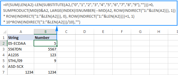
Unlike in all previous examples, the result of this formula is number. To make sure of this, just notice the right-aligned values in column B and truncated leading zeros.
Tip. In Excel 365 - Excel 2019, there is a much simpler solution with the help of the TEXTJOIN function. Please see How to remove text and keep numbers.
Extract number from text string with Ultimate Suite
As you have just seen, there is no trivial Excel formula to pull number from a text string. If you have difficulties with understanding the formulas or tweaking them for your data sets, you may like this simple way to get number from string in Excel.
With our Ultimate Suite added to your Excel ribbon, this is how you can quickly retrieve number from any alphanumeric string:
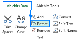
- Go to the Ablebits Data tab > Text group, and click Extract:
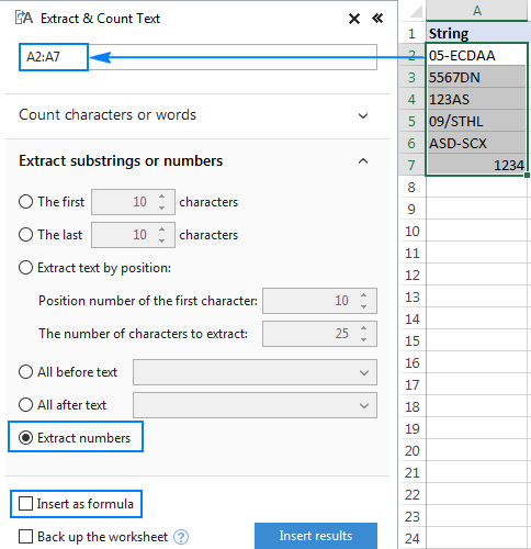
- Select all cells with the source strings.
- On the Extract tool's pane, select the Extract numbers radio button.
- Depending on whether you want the results to be formulas or values, select the Insert as formula box or leave it unselected (default).
My advice is to select this box if you want the extracted numbers to update automatically as soon as any changes are made to the source strings. If you want the results to be independent on the original strings (e.g. in case you plan to remove the source data at a later point), then do not select this box.
- Click the Insert Results button. Done!
Like in the previous example, the results of the extraction are numbers, meaning you are free to count, sum, average, or perform any other calculations with them.
In this example, we've chosen to insert the results as values, and the add-in did exactly what was asked for:
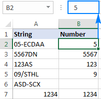
If the Insert as formula checkbox was selected, you'd observe a formula in the formula bar. Curious to know which one? Just download Ultimate Suite's trial and see for yourself :)
Available downloads
Excel Extract Number - sample workbook (.xlsx file)
Ultimate Suite - trial version (.exe file)
 by
by
557 comments
Hi there. I appreciate the detailed approach to this challenge. I have the following text:
"[SW] 183 Patterson -- WAN1 DOWN -- PL"
I'm using the formula above "How to get number from any position in a string"
Instead of returning 183, it returns 1831 - adding an extra 1 at the end?
Another text:
[SW] 016 Bremerton -- Router DOWN -- PWR" returns 16 instead of 016?
All thoughts are very much appreciated.
Hello!
Your first example has 4 digits. All of them are returned by the formula. In the second example, the result is returned as a number, not as text. Excel removes leading zeros from numbers.
To extract numbers as text, try this formula:
=CONCAT(IF(ISNUMBER(--MID(A2,ROW($1:$100),1)),MID(A2,ROW($1:$100),1),""))
You can also extract numbers from text using regular expressions (Regex). I recommend this tutorial with examples: Regex to extract number from string.
Hi,
Thanks for sharing this very helpful code. I have a problem with number that has digit like 1.5 or 3.70 it turn to 15 and 370. Could you please guide me how to fix that :)
Thanks again!
Hello!
To extract a number with a decimal separator from text, use the formula:
=CONCAT(IFERROR(MID(A2,(ISNUMBER(--MID(A2,ROW(INDIRECT("$1:$"&LEN(A2))),1))+ (MID(A2,ROW(INDIRECT("$1:$"&LEN(A2))),1)="."))* ROW(INDIRECT("$1:$"&LEN(A2))),1),""))
I hope I answered your question.
This formula looks so close to what I need. I'm wondering if someone wouldn't mind showing me how to tweak it to suit my requirement?
We receive many payments each day with various narratives, I would like to automatically identify references which are 7 digit number beginning with "13" or "14". Examples below and to the right is the currently formula result.
I am using this formula, essentially copied from above comments and info - I think I need to have the result only report back when the sequence beginning with "13" or "14" is 7 digits in length.
Any thoughts?
=IF(SUM(LEN(A22)-LEN(SUBSTITUTE(A22, {"13","14"}, "")))>0, SUMPRODUCT(MID(0&A22, LARGE(INDEX(ISNUMBER(--MID(A22,ROW(INDIRECT("$1:$"&LEN(A22))),1))* ROW(INDIRECT("$1:$"&LEN(A22))),0), ROW(INDIRECT("$1:$"&LEN(A22))))+1,1) * 10^ROW(INDIRECT("$1:$"&LEN(A22)))/10),"")
PAYMENT FROM MR SIMON ZHAO LPSPR 8486 No result-correct
TRANSFER 1322500 midas prch FROM SOON LEGAL 1322500-Correct
TRANSFER Ref 1401272 Susann FROM J BOGAN 1401272-Correct
PAYMENT FROM MS NILU JONCHHE Lot 136/Carseldine + Lot136/Carseldine 136136 - Incorrect
0491400550 HORNSBY 491400550-Incorrect
TRANSFER 1398031 FROM SETTLEMENT FUNDS 1398031-Correct
Thank you
Hi!
To extract 7 digit number beginning with “13” or “14” from text, you can use the formula
=(MID(A2,SEARCH(" 13",A2)+1,7)* ISNUMBER(--MID(A2,SEARCH(" 13",A2)+1,7)))* ((--MID(A2,SEARCH(" 13",A2)+1,7)* ISNUMBER(--MID(A2,SEARCH(" 13",A2)+1,7))) > = 1000000)*(MID(A2,SEARCH(" 13",A2)+8,1)=" ")
For the number "14", replace "13" with "14" in the formula.
You can also use regular expressions to extract numbers from text.
At the link above you will find detailed explanations and examples of how to extract text and numbers from a string. Here is an example formula that will solve your problem:
=RegExpExtract(A1&" "; "\s[1][34]\d{5}\s")
I hope it’ll be helpful. If something is still unclear, please feel free to ask.
Hi, i need to extract a group of text from a cell, and sum them together. before i begin, i would like to clrify that, I am not an Excel pro user like accountant. I'm using it as a data link between AUTOCAD and EXCEL. so, please bear with me.
A B c
1 YES 1800/ 900/ 1200 X 500 3900
2 NO 600/ 100/ 300/ 20 X 15 0
YES and NO is in column A (row 1 and 2 respectively). while the number is in column B. and the sum will appear in column C next to each row. i'm looking for a formula to extract 1800, 900, and 1200 to sum it up into 3900 (1800+900+1200), and it only extract and sum it when the column A says "YES", and will not do the sum when A says "NO".
sorry, the sample text arrangement went wrong.
YES 1800/ 900/ 1200 X 500 = 3900
NO 600/ 100/ 300/ 20 X 15 = 0
sorry, the sample text arrangement went wrong.
ignore the A,B,C above the sample and 1,2 on the left
Hi!
You can extract numbers from text using substring functions with these formulas:
=--LEFT(B1,SEARCH("/",B1)-1)
=--MID(B1,SEARCH("/",B1)+1,SEARCH("/",B1,SEARCH("/",B1)+1)-1-SEARCH("/",B1))
=--MID(B1,SEARCH("/",B1,SEARCH("/",B1)+1)+1,SEARCH("X",B1)-1-SEARCH("/",B1,SEARCH("/",B1)+1))
Write the condition using the IF function:
=IF(A1="YES",=--LEFT(B1,SEARCH("/",B1)-1),"")
General formula for three numbers with condition:
=IF(A1="YES",LEFT(B1,SEARCH("/",B1)-1)+ MID(B1,SEARCH("/",B1)+1, SEARCH("/",B1,SEARCH("/",B1)+1)-1-SEARCH("/",B1))+ MID(B1,SEARCH("/",B1,SEARCH("/",B1)+1)+1, SEARCH("X",B1)-1- SEARCH("/",B1,SEARCH("/",B1)+1)),"")
i see. Thanks for your help. i will need some times to explore what you shared with me. looking at the formula you gave, is killing my brain. lol. will get back to you how it goes.
Thanks again for sharing
Hey i have some problem.
My job is to extract number from a cell. A cell has 4 digits of randomly generated number (ABCD). So i want to automatically extract number A into one cell, B into one cell and the rest. and sometimes i need to extract 2 number from the same cell. is there a clean way to do it?
Hi!
To extract the first digit from a number, use the LEFT function.
LEFT(A1,1)
To extract the second digit use the MID function.
MID(A1,2,1)
Also, use MID to extract the third and all other digits.
MID(A1,3,20)
Look for the example formulas here: Excel substring functions to extract text from cell.
These functions extract a digits as text. To convert it to a number, use these guidelines: Turn text into number with mathematic operations.
I hope it’ll be helpful.
This was so helpful. I appreciate the effort of the team. Cheers!!!
This was very helpful, thanks!
Hi I hope you could help me!
I have some prices i need to extract...
?XIAOMI?
?Redmi 9A 32GB/2R 399.900 A,G??
?Redmi 10 64GB 744.900 B??
?Redmi 10 128GB 839.900 G??
?Poco X3 128GB/8R 949.900 G,A ??
?Poco X3 Pro 128GB/6R 909.900 N??
My question is... Is there a clean and simple way to only obtain the prices from this cellphones For example telling a formula to look for more than 4 consecutive numbers and extract them.
Look at this...
Redmi 9A 32GB/2R 399.900 A,G??
When I use a formula to look for only numbers it extracts 9322399900
I need something capable of skiping small number secuences and search for numbers bigger than (9A) (32GB) (2R) in this case 399000
I know that I can search for common characters like ($) $399000 to use text to columns.
But I have a wide range of providers that dont use any particular sign for me to use.
Hello!
To extract a group of numbers from a text, I recommend using a regular expression. You can find the examples and detailed instructions here: How to extract substrings in Excel using regular expressions.
Try this regex: "(\d+.\d+)(?!.*\d)"
I hope I answered your question. If something is still unclear, please feel free to ask.
Thanks a lot I have never heard of that so I will study about regex and tell you how it goes for me.
Thanks a lot. Both of your formulas worked great. Its amazing. I post some examples to Svetlana
Because some of my prices are in Millions and i was not able to interpret the formula to make it take into account bigger numbers. My knowledge of excel and english is very limited but I´m thankfull of your help. I´ve been doing this process the large way for about 2 years.
I could clean all of my data to have numbers without any signs. Example:
iPhone 13 128GB 5000000
iPhone 13 Pro 246GB 4500000
iPhone 12 Pro Max 512GB 3650000
Thanks in advance to all of you for your great work!
Hi Simon,
In case your prices have various delimiters like in the sample below, then cleaning the data before using the Regex formula is indeed the most effective way. As you said, first you remove all the characters between the prices (. , ’ ). And then, extract a number containing 4 or more digits using this simple regex:
\d{4,}
Hello Simon,
The only solution I can think of is using regular expressions. For this, you will need to add a custom RegExpExtract function to your workbook - the code and the detailed instructions are on the above-linked page.
As for the regex pattern, I don't think searching for 4 consecutive numbers will work in your case, because the prices in your sample strings have a thousands separator (period). So, you can use the below regex to match a substring consisting of 1-3 digits, followed by a period (.), followed by 3 digits.
Pattern: \b\d{1,3}\.\d{3}\b
The above pattern will work for numbers ranging from 1.000 to 999.999. If your real dataset has a wider range of numbers, you'll have to adjust the pattern.
Thanks a lot I have never heard of that so I will study about regex and tell you how it goes for me.
It worked perfectly. Could you please help me adjust the pattern for millions. I tried to interpret your formula but i couldn´t understand which is the key to increment to millions
I got some examples
Store A Example
Poco X3 Pro 8/256 GB $1’050.000 N-A ??
Poco X3 GT 8/128 GB $1’230.000 ??
Poco X3 GT 8/256gb $1.340.000 ??Blanco
Store B Example
IPHONE 12 MINI 64GB
BLANCO
$2.880.000
IPHONE 12 MINI 128GB
ROJO
$3.100.000
IPHONE 12 64GB
BLANCO
$3.300.000
Store C Example
11 pro max 256gb $4.200.000 negro????
12 64gb $3.350.000 blanco verde negro????
12 128gb $3.580.000 negro verde????
12 pro max 256gb $5.100.000 azul????
Store D Example
POCO X3 GT 8/128 AZUL Y BLANCO
$1’399.000??
MI 10T LITE 6/128GB AZUL
$ 1.235.000??
MI 11 LITE 5G 6/128GB NEGRO
$1’265.000??
Store E Example
Note 10 pro 128gb 6ram $1.329.000?? Azul
Note 10 5G 128gb 4ram $949.900?? Gris
Poco x3 pro de 128gb 6ram $ 924.900?? negro azul y bronce
Poco x3 pro de 256GB 8ram $1.059.900?? Negro y azul
Poco x3 GT 128gb 8ram $1.249.900?? azul negro y blanco
There are like 15 stores sending prices over WhatsApp I would love to understand how to adjust the pattern in the most efficient way. I don´t have any problem cleaning the data before using the Regex Formula. I mean replacing... ( . , ’ ) all the characters between my prices.
Hello!
Try a regular expression like this:
(\d+.\d+.\d+)(?!.*\d)
Hope this is what you need.
Hello Mr.Alexander Could you help me please I have example as below
LG-101+CC100+S+22 11 21+625+3
LG-101+CC100+S+22 11 21+625+300
LG-101+CC109+M+22 11 21+609+220
LG-76-2+92C+S+22 11 21+618+1140
and I want to get only value after + at the end of the cell like below
3
300
220
1140
Hi!
Read the first paragraph of this article carefully. There is an answer to your question.
It's works. You save my day.
How to match the last five numbers of the 10 figure number or string
Hello!
To get the last 5 numbers, use the RIGHT function as described in this article.
I'm trying to extract number and the text attached to it, lets say I have a list of items with different sizes as 200ml & 300ml, I want to extract 200ml 300ml from the cell, and also remove it from the source cell, is there any way with or without your tool to do this?
Thank you very much!
Hi!
I cannot guess what is written in your data. Therefore, I can not offer a solution. Use the SEARCH function to find values.
Perhaps something like this:
=IF(ISNUMBER(SEARCH("200ml",A1)),"200ml","")
You can only remove some of the text from a cell using a VBA macro.
What went wrong here?
A2: 10-Hour Orchid Class
B2: =LEFT(A2, MATCH(FALSE, ISNUMBER(MID(A2, ROW(INDIRECT( "1:"&LEN(A2)+1)), 1) *1), 0) -1)
Evaluation:
=LEFT(A2, MATCH(FALSE, ISNUMBER(MID(A2, ROW(INDIRECT( "1:"&LEN(A2)+1)), 1) *1), 0) -1)
=LEFT(A2, MATCH(FALSE, ISNUMBER(MID(A2, ROW(INDIRECT( "1:"&20+1)), 1) *1), 0) -1)
=LEFT(A2, MATCH(FALSE, ISNUMBER(MID(A2, ROW(INDIRECT( "1:"&21)), 1) *1), 0) -1)
=LEFT(A2, MATCH(FALSE, ISNUMBER(MID(A2, ROW(INDIRECT( "1:21")), 1) *1), 0) -1)
=LEFT(A2, MATCH(FALSE, ISNUMBER(MID(A2, ROW(INDIRECT($1:$21)), 1) *1), 0) -1)
=LEFT(A2, MATCH(FALSE, ISNUMBER(MID(A2, 1, 1) *1), 0) -1)
=LEFT(A2, MATCH(FALSE, ISNUMBER("1" *1), 0) -1)
=LEFT(A2, MATCH(FALSE, ISNUMBER(1), 0) -1)
=LEFT(A2, MATCH(FALSE, TRUE, 0) -1)
=LEFT(A2,#N/A -1)
=LEFT(A2,#N/A)
=#N/A
Hi!
I can't guess what your problem is.
ROW(INDIRECT( "1:"&LEN(A2)+1)) seems to not be evaluating to a sequence, just the number 1 (1.00 to be precise). But I don't know why. On another machine, this formula worked.
Hi!
See the difference between Excel versions and program settings.
u can use below one
=LEFT(A2,MATCH(FALSE,ISNUMBER(MID(A2,ROW(INDIRECT("1:"&LEN(A2))),1)+0),0)-1)
u can use below one with ctrl+shift+Enter
=LEFT(A2,MATCH(FALSE,ISNUMBER(MID(A2,ROW(INDIRECT("1:"&LEN(A2))),1)*1),0)-1)+0
I would like to make a formula that can Extract the individual numbers from the example below. The numbers will change on either side of the x. My goal is to extract the single digits and place them in their own sell. The example below will be located in one cell group together again the digits will change depending on information.
Example one .75 x 2 x 31
Example two. 4 x 89 x 107
.75 x 2 x 31 >>>> 0.75 2 31
4 x 89 x 107 >>>> 4 89 107
Hello!
You must split the text string at the "x" delimiter. Read the guidelines in this article.
Replace (SpaceXSpace) with (Single ot Multiple Space/s).
Hi All,
I have a sentence in one cell and want to extract all the values in multiple columns e.g.
Data in cellA1
Total sales increased $58.9 billion or 4.5% from October 31, 2020 due increase in demand medical products by $15.2 billion or 2%
I want all the Monetary values and % in different cells
B1 = 58.9
C1 = 4.5
D1 = 15.2
E1 = 2
Hi!
All possible recommendations are described in the article above.
Hey Alex, I have tried those..but thats not helpful..as those are also extracting 31 and 2020 which is not relevant..Could you please help me on the same
Hi!
If you have a pattern in your data, you can write a formula that will remove the date. Only all numbers can be extracted from the text.
I Textjoin row of cells. Only one contains date and time. Other cells, if NOT blank, contains text including numbers NOT dates.
Textjoin works but date and time is now in serial format.
How to convert that serial format within the Textjoin Output back to date and time?
I solved by extract 9 consecutive digits (including decimals) but hope better solution such as avoiding indirect...
=
MAX(
IFERROR(
IF(
LEN(
VALUE(
1*
MID(
$A$2,
ROW(INDIRECT("1:"&(LEN($A$2)-9))),
9)
)
)=9,
VALUE(
1*
MID(
$A$2,
ROW(INDIRECT("1:"&(LEN($A$2)-9))),
9)
),
""),""))
Hello!
Use the TEXT function to convert date to text.
=TEXTJOIN(" ",TRUE,TEXT(A1,"dd-mmm-yyyy"),B1,C1,D1)
Hi there,
Is there one formula that can turn the below into "h:mm:ss"? The data source can be in below formats
3h 31m
8h
51m 3s
Hi!
I am looking for a formula to return the first two digits of an account number
ie account number1 =1212341234567000
account number2 =0812341234567000
I want to be able to return just 12 for account 1 and 08 for account 2. (I then want to assign a name for each of these first two digits).
Please help :)
=LEFT(CELLNUMBER1;2)
Hello, thanks for your help! Can you please help with the following:
Each row corresponds to one cell:
53QBx13 bunches Limonium Piña Colada 70cm (10st) $2.60
13QBx13 bunches Limonium Piña Colada 80cm (10st) $2.80
8EBx10 bunches Limonium Oshi Pink BQT 60cm (20st) $3.50
I need to extract in columns the following:
Column 1
53
13
8
Column 2
QB
QB
EB
Column 3
13
13
10
Column 4
Limonium Piña Colada
Limonium Piña Colada
Limonium Piña Colada
Column 5
70
80
60
Column 6
$2.60
$2.80
$3.50
Is this possible?
Thanks!
Hello!
Your problem cannot be solved with a formula. Please have a look at this article — How to split data in Excel cell with the Split Text tool.
Hi Alexander! I just wanted to thank you so very much for your time and effort in assisting me.
In case you were curious, I was able to extract and add the numbers that I wanted by using this VBA code along with "SUMNUMS":
Function SumNums(pWorkRng As Range, Optional xDelim As String = " ") As Double
Dim arr As Variant
Dim xIndex As Long
arr = Split(pWorkRng, xDelim)
For xIndex = LBound(arr) To UBound(arr) Step 1
SumNums = SumNums + VBA.Val(arr(xIndex))
Next
End Function
Thanks again, you are amazing!
Good day! I am trying to extract and add the number of pages in each line of the following example:
(1 x Stapled): 1 x Ldgr/C
(1 x Stapled): 4 x Ltr/D
(1 x Stapled): 17 x Ldgr/C
(1 x Stapled): 26 x Ldgr/C/D; 1 x Ldgr/C
(1 x Stapled): 16 x Ldgr/C/D; 1 x Ldgr/C
(2 x Stapled): 32 x Ldgr/C/D; 2 x Ldgr/C
(1 x Stapled): 9 x Ltr/D; 7 x Ltr/C/D; 1 x Ltr
(1 x Stapled): 1 x Ltr/C
Might you be able to assist with a formula? Much appreciated!
Hi!
Sorry, it's not quite clear what you are trying to achieve.
What does the “(1 x Stapled): 1 x Ldgr/C” phrase mean?
Describe in detail what problem you have, and I will try to help you.
Hi Alexander! Thanks so much for the quick reply. This is data from our photocopier usage. Each line is a print job; the first number is how many staples were used, followed by how many pieces of paper, letter (ltr) or ledger (ldgr))size. I'm trying to extract the number of pages printed for each line and add them together.
I hope that helps! Please let me know if you need further details.
Hi!
Based on your description, it is hard to completely understand your task. However, I’ll try to guess and offer you the following formula:
=--MID(A1,SEARCH(":",A1,1)+1,SEARCH("x",A1,SEARCH(":",A1,1))-SEARCH(":",A1,1)-1)
You can also use Split Text tool with mask
*:*x*
It is available as a part of our Ultimate Suite for Excel that you can install in a trial mode and check how it works for free: https://www.ablebits.com/files/get.php?addin=xl-suite&f=free-trial
Thanks so much! This is sooo close to what I'm looking for. :) I'm sorry I'm not explaining it very well...
If you look at this line:
(1 x Stapled): 1 x Ltr/C/D; 7 x Ltr/D; 1 x Ltr
The result I'm looking for is "9".
I hope that makes it more clear! You are certainly a wizard. Thank you so very much for your time and assistance!
Hello!
In the text
(1 x Stapled): 1 x Ltr/C/D; 7 x Ltr/D; 1 x Ltr
there are numbers 1 1 7 1
Which ones do you sum to get 9?
Hi! The first number is the number of staples, so I do not want to add that one; just the three following numbers which are number of pages used. :)
Hope that helps! Thanks so much!
Hello!
If I got you right, the formula below will help you with your task:
=SUM((IF(ISNUMBER(--MID(MID(A1,14,100),ROW($1:$100),1)),--MID(MID(A1,14,100),ROW($1:$100),1),"")))
I hope my advice will help you solve your task.
Hi, how to extract numbers in middle of Unicode strings, example "2 – 이 (i)"? Thanks Ahead!
5KM (1) Back to Basics
>21KM Sky's the Limit
Hi, I'm amazed by Sir Alexander's superb excel skills. I'm just trying out my luck here hopefully sir can solve my problem. I would like to extract only the number '5' and '21'. I wonder it is possible. Thank you.
Hello!
Press CTRL + H. In the "Find what" field, write (*). Do not write anything in the "Replace with" field. Click "Replace".
Then use the formula from this article and comments. For example:
=TEXTJOIN("",TRUE,IFERROR(MID(A2,ROW(INDIRECT("1:"&LEN(A2))),1)*1,""))
I hope I answered your question.
Hi,
I have a spreadsheet of thousands in the following format
1. zvsnsnshs 2020DDE542134
2. sgenemene2020SHB6721
3. reenmennee 2020RTY409
I want to extract 2020DDE542134 in 1, 2020SHB6721 in 2 and 2020RTY409 in 3
2020 is followed by three letters but the number of digits thereafter vary.
Please assist.
Hello!
The formula below will do the trick for you:
=MID(A1,SEARCH("2020",A1,1),100)
I hope it’ll be helpful.
I use this to get numbers only from mixed Alpha Numeric strings
TEXTJOIN(“”,TRUE,IFERROR(MID(A2,ROW(INDIRECT(“1:”&LEN(A2))),1)*1,””))
Amazing formula and explanation. Thank you very much!
Hello,
How can i remove last numeric digit from a text numeric string e.g.
abc, adi, 23 fhve sihf ghr 98000
Thank you for this amazing formula!
=SUMPRODUCT(MID(0&A2, LARGE(INDEX(ISNUMBER(--MID(A2, ROW(INDIRECT("1:"&LEN(A2))), 1)) * ROW(INDIRECT("1:"&LEN(A2))), 0), ROW(INDIRECT("1:"&LEN(A2))))+1, 1) * 10^ROW(INDIRECT("1:"&LEN(A2)))/10)
It works almost perfectly, however I would like to separate the different number sets with a space.
e.g.
returned value with formula: 5468751013
desired return value: 546875 1 0 13 (number sets vary)
Regards
Donald
Hello!
If you want to extract groups of numbers from the text and separate them with a space, use this formula:
=SUBSTITUTE(TRIM(CONCAT(IF(ISNUMBER(--MID(A2,ROW($1:$94),1)),MID(A2,ROW($1:$94),1)," ")))," "," ")
Hope this is what you need.
Wow! That worked perfectly!
Greatly appreciate this support!
I find this thread quite amazing.
What I offer below may be a solution to a one-off problem as no-one else describes anything similar. But perhaps I am not the only one so here goes.
When I scraped a table from the following site:
https://en.wikipedia.org/wiki/List_of_countries_by_net_migration_rate
- I found columns of numbers displayed in Excel as either regular positive numbers, aligned right, or negative numbers as text, aligned left. I tried all the techniques recommended for converting text to number but nothing worked. So in frustration I converted them all manually, hardly a practical solution for a large database.
Then it dawned on me that it must be the actual "-" character which was causing the problem. I discovered there are online Unicode character identifiers, one of which I used to identify how these negative characters were different. The "-" for a regular negative number identified as "U+002D : HYPHEN-MINUS {hyphen or minus sign}". The problem character identified as "U+2212 : MINUS SIGN". When I used Ctrl-H, find and replace-all in Excel, all the negative text numbers instantly converted to regular numbers, aligned right, no further action needed.
BR_GID/908764_JK2
what is the formula to get only 908764 number .
Hi,
Please check the formula below, it should work for you:
=LEFT(SUBSTITUTE(TRIM(CONCAT(IF(ISNUMBER(--MID(A1,ROW($1:$94),1)), MID(A1,ROW($1:$94),1)," ")))," ","-"), SEARCH("-",SUBSTITUTE(TRIM(CONCAT(IF(ISNUMBER(--MID(A1,ROW($1:$94),1)), MID(A1,ROW($1:$94),1)," ")))," ","-"),1)-1)
I hope it’ll be helpful.
Hi,
I have a spreadsheet of a couple of thousand lot plans in the format of
103SP122202
10SP133260
1RP43701
They are always numbers followed by letters followed by numbers.
I am looking for a formula to return all the numbers before the first letter and place in a column
103
10
1
Then a formula to return all the letters, and the numbers after the letters to place in another column
SP122202
SP133260
1RP43701
how would i achieve this?
Hello!
Write your value in cell A1. To extract the text, write the formula in B1.
=SUBSTITUTE((CONCAT(IF(NOT(ISNUMBER(--MID(A1,ROW($1:$94),1))), MID(A1,ROW($1:$94),1),"")))," ","")
To extract the first number, write the formula in C1.
=LEFT(A1,SEARCH(B1,A1,1)-1)
To extract the second number, write the formula in D1.
=RIGHT(A1,LEN(A1)-SEARCH(B1,A1,1)-1)
I hope I answered your question. If something is still unclear, please feel free to ask.
Hi Alexander,
Thank you very much for replying with a solution, it works very well.
Is it possible to alter =RIGHT(A1,LEN(A1)-SEARCH(B1,A1,1)-1) to keep SP122202 together in a cell and not separated?
Regards
Andrew
Hi,
Please try the following formula:
=B1&RIGHT(A1,LEN(A1)-SEARCH(B1,A1,1)-1)
or
=RIGHT(A1,LEN(A1)-SEARCH(B1,A1,1)+1)
Hi,
The second formula worked perfectly,
Thank you very much.
Regards
Andrew
I've been an advanced Excel user for 10+ years. It's pretty rare these days but when I hit a wall I eventually search for something online and I'm amazed, how many of those times I've ended up on one of Svetlana's posts, like 50+. I'm a big fan of hers! Joshua
Hi Team,
I want below number to be extract from below given sentence.
Q. 1 : "GL CASH DIPOSITED DONE BY ONE DATE IS 05/10/2020 02771600241 [AccountID: 123456767"
I want the answer should be "02771600241"
Q2: CASH DEPOSITED IN TRANSACTION ID - 02801900536 [AccountID: 1257895333 Account Name: Cas
I want the answer should be " 02801900536 "
Hi,
If I got you right, the formula below will help you with your task:
=TRIM(RIGHT(SUBSTITUTE(TRIM(RIGHT(SUBSTITUTE(LEFT(A1,SEARCH(" [",A1,1)),"-",REPT(" ",20)),20))," ",REPT(" ",20)),20))
What if I have multiple potential phone numbers in a free-form field and want them to extract, but be separated by a delimiter? Working from a DB extract where the most useful phone numbers are entered free-form with other miscellaneous tidbits like this:
UserName 1234567890 Location 0987654321 OtherInfo
OtherInfo 1234567890 Location
M 1234567890 C 0987654321
Location 1234567890 0987654321
While your formula works great for extracting the numbers, it's resulting in strings like this now 12345678900987654321, which I would then need to split back up. Not all #s are 10 digits. Some have only 7 and others are international.
Hello!
You have not written what result you want to get. Therefore, I can only recommend this article - Custom Excel number format.
If something is still unclear, please feel free to ask.
Thanks for the formula, its really helpful and time saving
Hi,
If i need to do the sum of the below 2 columns which has number and a percentage in same cell, how do i do this?
Could you please help. Thanks a lot.
4 (100%)
5 (83%)
Hi,
What result do you want to get exactly? Your question is not entirely clear, please specify.
Thank you for replying.
COlumn A Column B
Total test runs Total test executed
4 4 (100%)
6 5 (83%)
------------------------------------------------------
10 9 (91.66%)
In column B, I want to get the total no of executed test cases ( 4+5). Also I want to get the average percentage of column B v/s Column A total count.
Hello!
To convert text string "4 (100%)" to number 4 use the formula
=--REPLACE(B2,SEARCH("(",B2,1),10,"")
I hope it’ll be helpful.
Hi Alex,
Problem description
TXT_TXN_DESC Required field
NEFT Cr-UTIB0000231-SIVA C-JANA SMALL FINANCE BANK-AXIR210011779565 AXIR210011779565
RTGS Cr-HDFC0000240-LIGHTMICROFINANCEPVTLTD-JSFBCollectionAccountMSE-HDFCR52021010166833120 HDFCR52021010166833120
NEFT SBIN521001912911-Mrs GOPA BHATACHARJEE-JANA SMALL FINANCE BANK LTD SBIN521001912911
30768647394421 KKBKR52021010200888475 KKBKR52021010200888475
33598650000698 20210102 IOBAN21002635205 IOBAN21002635205
30098850001352 P002210081154581 20210102 P002210081154581
What formula will work for to segregate an UTRNs to new column, please suggest.
Hi,
What do you want to calculate exactly? Your question is not entirely clear, please specify.
Is this text from one cell or from several? How do you want to split it? Give an example.
Hi,
I have used your formula above for extracting numbers from the left of a string [=LEFT(C738,SUM(LEN(C738)-LEN(SUBSTITUTE(C738,{"0","1","2","3","4","5","6","7","8","9"},""))))] but it is not returning the expected result:
* String - 198503_NA_ST17 9UQ
* Expected result - 198503
* Actual result - 198503_NA
If you could give me any indication as to where I have gone wrong it would be very much appreciated.
Kind regards,
Matt
Hello!
Please try the following formula:
=LEFT(A2,MATCH(FALSE,ISNUMBER(--MID(A2,ROW($1:$94),1)),0)-1)
Hope this is what you need.
Hi Alexander,
Thanks for your help but unfortunately that is returning #N/A.
I changed the cell reference to C113 to suit where I am extracting the data from (I am extracting it into cell A113) and changed ROW references to $5:$475 as those are the rows my full data set sits in.
Have I gone wrong somewhere making those changes? I tried it without changing the ROW references but it still returns #N/A.
Thanks again for your help.
Matt
Hi,
No need to change absolute references.
=LEFT(C113,MATCH(FALSE,ISNUMBER(--MID(C113,ROW($1:$94),1)),0)-1)
If you are using Excel 2019 and below, enter this formula as an array formula. In Excel 365, you can type as usual using the Enter key.
Thanks for the site, I reference often.
Here is my new hack for this: (OFFICE365 Only)
=LET( A, MID($J2,ROW(INDIRECT("1:"&LEN($J2))),1),
F, FILTER(A, ISNUMBER(A*1)),
CONCAT(F)
)
Hello, plz
Can anybody help me out.
I have 26(4),5(7),9(10) in A1.
I want to extract the numbers like this:
26 in B1
4 in C1
5 in D1
7 in E1
9 in F1
10 in G1
Plz Help.
Hi,
We have a tool that can solve your task in a couple of clicks - Abledits Data - Split Text. It is available as a part of our Ultimate Suite for Excel that you can install in a trial mode and check how it works for free.
Good day,
what formula will work best, if you want to create a register list. That when you type an employee's pers number all the personal info pulls through eg. name, surname, job title and workplace. I have the master data sheet but want to make my life easier when reporting on other related reports.
Hi, I used the formula to extract number from beginning of strings :
=LEFT(A2,SUM(LEN(A2)-LEN(SUBSTITUTE(A2,{"0","1","2","3","4","5","6","7","8","9"},""))))
to extract
2A 1234521
it was supposed to extract 2, but instead it extract
2A 12345
Why is that? Please help.
Hi Shay,
To extract a number only from the beginning, please use this formula:
=LEFT(A2, MATCH(FALSE, ISNUMBER(MID(A2, ROW(INDIRECT( "1:"&LEN(A2)+1)), 1) *1), 0) -1)
Hello
I would like to extract only those number which has tin written in front. can someone help me with formula.
Goodman Fielder tin500766109 FOODMEA072 Chicken Thighs Normal (CTN/7.5KG)
Foods Pacific Ltd tin 500546606 FOODDAI074 Cheese Mozzarella Grated 5 Star Gold (CTN/ 2x5KG)
Tappoo tin500618105 BEVCIDER004 Cider Pear Isaac's (CTN/ 12x330ml)
Tappoo tin500618105 BEVCIDER005 Cider Apple Isaac's (CTN/ 12x330ml)
Satish Kumar Marketing tin 113065604 FOODVEG074 VegAlfalfa Sprout Imported (Punnet)
Hello Reader, just another comment . . .
But need you + any assistants, to know VERY VERY sincere appreciation for such brilliant compilation of commitment to others having a success using sheets, over many years ! !
I only started when PC’s were 16K / 64K we could do 255 x 255 single sheets . . . Oh, how it’s changed.
THANKYOU & hopefully your future plans for site develop how you wish.
Best Regards,
Lee_ an Aussie
ps. ;-)
Hello,
I would like to extract the phone numbers from this cell.
7. UZOUKWU, PRINCE ROYCE 0803 743 5119-MUM/0803 275 9140-DAD
I have a long spreadsheet of names & the positioning of the phone numbers are not in the same place.
However I will separate these phone numbers in 2 cells.
Hello!
If the phone number always has the same number of digits, you can try these formulas:
=MID(A1,SEARCH("-",A1,1)-13,13)
=MID(A1,SEARCH("-",A1,SEARCH("-",A1,1)+1)-13,13)
I hope I answered your question. If something is still unclear, please feel free to ask.
The first one worked, for the first phone numbers and the 2nd pulled the 2nd phone number.
Thank you so much.
Hi alexander,
How do i extract number from
1 - 123, Singh Petrol Pump, Bishrampur, 497226, 36
2 - Company, 123, 123, 788031, 123
3 - 234, Danapur Maruti Suzuki Agency, Gopalganj, 841427, Bihar
4 - Plot No RM-126,R & C Zone,, MIDC INDL. Area, Butibori. Dist Nagpur, 441122, 27- Maharashtra
FOR 1ST ROW I WANT 497226
FOR 2ND ROW I WANT 788031
FOR 3RD ROW I WANT 841427
FOR 4TH ROW I WANT 441122
Please let me know the formula
Hello!
You are using commas as word separators. You can extract the penultimate word using the formula —
=TRIM(MID(A1,FIND("*",SUBSTITUTE(A1,",","*",LEN(A1)-1 -LEN(SUBSTITUTE(A1,",",""))),1)+1, FIND("*",SUBSTITUTE(A1,",","*",LEN(A1)- LEN(SUBSTITUTE(A1,",",""))),1)- FIND("*",SUBSTITUTE(A1,",","*",LEN(A1)-1 -LEN(SUBSTITUTE(A1,",",""))),1)-1))
Hope this is what you need.
Thank you Alexander
what if i want to get only 4 digit for example :
aadfnmm kadflk ZZ56 ladkkfiiss
alkliid kalkem 23 lsd 5675 llk,slkdk
thanks you
ILH-E-AC-030
ILH-E-AC-031
ILH-E-AC-032
ILH-E-AC-033
ILH-E-LO-003 SHT1
ILH-E-LO-003 SHT2
ILH-E-LO-027 SHT1
ILH-E-LO-027 SHT2
ILH-E-LO-027 SHT3
i want to extract this to other cell so it look like:
030
031
032
033
033
033
027
027
027
can someone tell me the formula to extract just the 3 digits number after the last "-" from left?
Hello!
I hope you have studied the recommendations in the tutorial above. It contains answers to your question.
I am trying to pull just $ amount with Decimals and commas in this sentence how would I do that
Paying total amount of $ 12,275.21
Thanks in advance
Thank you, it's works!
Working Fine.
=CONCAT(IF(ISNUMBER(--MID(A4,ROW($1:$93),1)),MID(A4,ROW($1:$93),1),""))
Using the formula
1orrange&2apple = 12 ( Answer getting now)
I need the answer as
1orrange&2apple = 3 ( it suppose to add up the numbers)