The complete guide on how to find and extract text from string between two characters or words in Excel and Google Sheets.
When working with long strings, you may often want to extract a specific part of them for closer examination. In Microsoft Excel and Google Sheets, there are several ways to get text between two characters or substrings. In this article, we'll discuss the fastest and most effective ones.
How to extract text between two characters in Excel
To extract text between two different characters, you can use this generic formula:
For example, to get text between parentheses from the string in A2, the formula is:
=MID(A2, SEARCH("(", A2)+1, SEARCH(")", A2) - SEARCH("(", A2) -1)
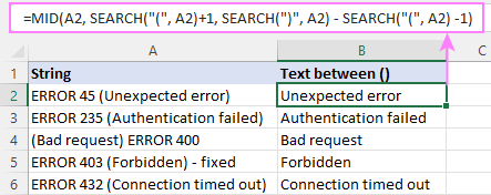
In a similar manner, you can extract text between braces, square brackets, angle brackets, and so on.
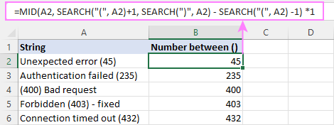
Useful tip! If you are dealing with numbers and want the result to be a number and not a numeric string, then additionally perform some arithmetic operation that does not change the result, e.g. add 0 or multiply by 1.
For example:
=MID(A2, SEARCH("(", A2)+1, SEARCH(")", A2) - SEARCH("(", A2) -1) *1
Please notice the default right alignment of the extracted values in cells typical for numbers:
How this formula works
The base of this formula is the MID function that pulls a given number of characters from a string, starting at a specific position:
Text is the cell containing the original string (A2).
The starting position (start_num) is the character that immediately follows the opening parenthesis. So, you find the position of "(" using the SEARCH function and add 1 to it:
SEARCH("(", A2) +1
To figure out how many characters to extract (num_chars), you locate the position of the closing parentheses and subtract the position of the opening parentheses from it. Additionally, you subtract 1 to leave out the second parentheses:
SEARCH(")", A2) - SEARCH("(", A2) -1
Having all the necessary details, the MID function brings you exactly what you want – text between parentheses in our case:
MID(A2, 19, 2)
As MID is a text function, it always produces a string, even if the extraction only includes numbers. To get a number as the final result, we multiply MID's output by one or add zero to it. If you are extracting text, this operation is not required.
Extract text between two strings / words in Excel
To pull text between two strings or words, the formula is quite similar to the one discussed above. Only a couple of different adjustments are needed: to remove the delimiter-words from the final result, you add and subtract the length of the words themselves returned by the LEN function:
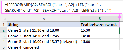
For example, to extract substrings between the words "start" and "end", the formula is:
=IFERROR(MID(A2, SEARCH("start ", A2) + LEN("start "), SEARCH(" end", A2) - SEARCH("start ", A2) - LEN("start ")), "")
Tips:
- To avoid leading and trailing spaces in the results, include a space after word 1 such as "start " and before word 2 such as " end". Alternatively, you can use the TRIM function to get rid of extra spaces.
- If one or both of the specified words are not found in the original string, the formula will return the #VALUE! error. To catch that error and replace it with an empty string (""), use the IFERROR function like shown in the above example.
Get text between two instances of the same character in Excel
To extract text from a string between two occurrences of the same character, the generic formula is:
For example, to extract text between double quotes from the string in A2, you enter this formula in B2:
=MID(A2, SEARCH("""", A2) +1, SEARCH("""", A2, SEARCH("""",A2) +1) - SEARCH("""", A2) -1)
Please pay attention to the way you search for a double quote in Excel. Between the outer quotes, another set of quotes is entered. The first quote is used to escape a special meaning of the second quote so that "" in between the outermost quotes stands for a single double quote.
Another way to supply a double quote (") to an Excel formula is by using the CHAR function with the code number 34.
=MID(A2, SEARCH(CHAR(34), A2) +1, SEARCH(CHAR(34), A2, SEARCH(CHAR(34),A2) +1) - SEARCH(CHAR(34), A2) -1)

How this formula works
The first two arguments of this MID formula raise no questions:
- A2 is the text string to search, and
- SEARCH("""", A2) +1 is the starting number, i.e. the position of the first quote +1.
The trickiest part is calculating the number of characters to extract (num_chars):
First, we find the position of the second quote by nesting one SEARCH function within another.
SEARCH("""", A2, SEARCH("""",A2) +1)
From the position of the 2nd quote (in A2 it's 27), you subtract the position of the 1st quote (in A2 it's 10), and then subtract 1 to exclude the quote itself from the result:
SEARCH("""", A2, SEARCH("""",A2) +1) - SEARCH("""", A2) -1
The above formula returns 16, which is the last missing piece of a puzzle the MID function needs:
=MID(A2, 10+1, 16)
Simply put, MID searches the cell A2 starting from the character after the 1st quote (10+1) and returns the next 16 characters.
Case-sensitive Excel formula to extract text between characters
As you probably know, in Microsoft Excel there are two functions to search strings: SEARCH (case-insensitive) and FIND (case-sensitive).
In situation when the delimiter is a letter in a specific case, just use FIND instead of SEARCH. To illustrate the difference, let's compare the two formulas below.
From the string in A2, suppose you want to extract a number between two uppercase letters "X".
The SEARCH function works incorrectly in this case because it does not distinguish between "x" and "X":
=MID(A2, SEARCH("X", A2) +1, SEARCH("X", A2, SEARCH("X",A2) +1) - SEARCH("X", A2) -1) +0
As the result, the text between "x" is extracted, and not between "X" that we are looking for:

While the case-sensitive FIND function works beautifully:
=MID(A2, FIND("X", A2) +1, FIND("X", A2, FIND("X",A2) +1) - FIND("X", A2) -1) +0
And brings exactly the result we need:

Extracting text between characters in Excel 365
In Excel 365, you can get text between characters more easily by using the TEXTBEFORE and TEXTAFTER functions together.
For example, to extract text between parentheses, the formula is as simple as this:
=TEXTBEFORE(TEXTAFTER(A2, "("), ")")
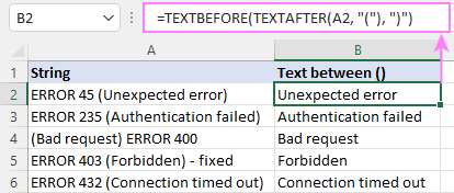
This formula also works nicely for extracting text between two occurrences of the same character.
For instance, to get text between double quotes, the formula takes this form:
=TEXTBEFORE(TEXTAFTER(A2, """"), """")
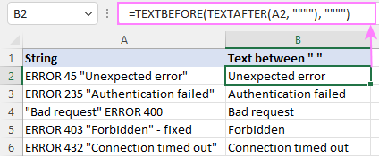
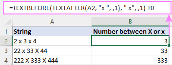
By default, both the TEXTAFTER and TEXTBEFORE functions are case-sensitive. To disable case-sensitivity, you set the 4th argument (match_mode) to 1 or TRUE.
For example, the case-insensitive formula below recognizes both the lowercase "x" and uppercase "X" as the delimiter:
=TEXTBEFORE(TEXTAFTER(A2, "x ", ,1), " x", ,1) +0
How this formula works
Working from the inside out, you use the TEXTAFTER function to extract text after the opening parentheses:
TEXTAFTER(A2, "(")
And serve the returned substring to TEXTBEFORE, asking it to find the closing parentheses in that substring and return the text before it.
TEXTBEFORE("Unexpected error)", ")")
Done :)
Get text between two characters in Google Sheets
To find text between two characters in Google Sheets, you don't need to reinvent the wheel :)
The MID SEARCH combinations used in Excel work flawlessly in Google spreadsheets too.
For instance, to get text between brackets, the formula is:
=MID(A2, SEARCH("[", A2)+1, SEARCH("]", A2) - SEARCH("[", A2) -1)

To extract text between two commas, this is the formula to use:

That's how to extract text between two characters or words in Microsoft Excel and Google spreadsheets. I thank you for reading and hope to see you on our blog next week!
Practice workbooks
Extract text between characters in Excel (.xlsx file)
Get text between characters in Google Sheets (online sheet)
 by
by
26 comments
A great way to convert US dates to UK format
date in i4
=DATEVALUE(TEXTBEFORE(TEXTAFTER(I4,"/"),"/")&"/"&TEXTBEFORE(I4,"/")&"/"&RIGHT(I4,4))
US date = 12/6/2024
TEXTBEFORE(TEXTAFTER(I4,"/"),"/") This produces the day
&"/"& This produces the separator
TEXTBEFORE(I4,"/") this produces the month
RIGHT(I4,4) this produces the year if 4 digits
will produce 06/12/2024 when formatted as a date.
Hello,
I have a string of book details in the following format:
(Word Count) Title [Series Name] [Author Name]
I was able to extract the Series Name with this:
=MID(A1:A5, SEARCH("[", A1:A5)+1, SEARCH("] [", A1:A5) - SEARCH("[", A1:A5) -1)
However, the following formula was unsuccessful in extracting the Author Name:
=MID(A1:A5, SEARCH("] [", A1:A5)+1, SEARCH("]", A1:A5) - SEARCH("] [", A1:A5) -1)
I'm using Google Sheets. Is there an alternate formula for this format?
Hello ks,
If you'd like to stick with MID, use this formula for Author Name:
=SUBSTITUTE(SUBSTITUTE(TRIM(MID(A1, FIND("]", A1) + 1, LEN(A1) - FIND("]", A1))), "[", ""), "]", "")
But there are 2 easier ways:
One with REGEXEXTRACT:
=REGEXEXTRACT(A1, "\[([^]]+)\]$")
Another with the Extract tool, you'll get to know it in this blog post.
This question inspired me to split names with variable number of parts into 3 columns. I use 365. The names have 2 to 5 parts so the number of delimiters, ie spaces, is variable.
Column A FIRSTname MIDDLEname(s) LASTname
Column B FIRSTname extract with =TEXTBEFORE(A2," ")
Column C MIDDLEname(s) can have 0-3 strings extract with =IFNA(TEXTBEFORE(TEXTAFTER(A2, " "), " ",-1),"") ==>> note IFNA leaves cell empty if there is no middle name
Column D LASTname extract with =TEXTAFTER(A2," ",-1)
John Allen Jones John Allen Jones
Sue Patty Alice Smith Sue Patty Alice Smith
Rose Petal Blue Purple Object Rose Petal Blue Purple Object
Joe franklin Joe franklin
It would be REALLY helpful & much clearer if you didn't use parentheses or quotation marks (or any non-letter character that might be misinterpreted as PART of the prescribed formula) in your examples. It's so confusing because both parentheses & quotation marks are required in the formula! (an actual lol from me)
Extracting text between characters in Excel 365:
TEXTBEFORE(TEXTAFTER(A2, "("), ")")
and
=TEXTBEFORE(TEXTAFTER(A2, """"), """")
maybe use TEXTBEFORE(TEXTAFTER(A2, "@"), "#")
bankers like @yield# not people
to extract the word yield
especially since you put this without the quotations marks:
TEXTBEFORE(TEXTAFTER(cell, char1), char2)
What mods do I need to make if the enclosing characters are the same, please?
e.g. the column contains:
For 0 @I842@ INDI
I need the text between the @ signs. I can do it with two formulas but can I do it in one?
Regards
Paul
Hello Paul,
Do you work in Excel or Google Sheets?
Hi
whats the formula for this
for example i have this
(tu-35hg) sfdgj65hmn
(mt657) hnbdbhd (fghjfj) (dfhghj)
(jrutnb) dfhgdhd (yju56)
(23435) fhduh
want the result like this
sfdgj65hmn (tu-35hg)
hnbdbhd (fghjfj) (dfhghj) (mt657)
dfhgdhd (yju56) (jrutnb)
fhduh (23435)
(whats between characters in the first of the sentence become the last)
Thanks a lot
you can just replace (*) by blank value. you will get the results.
hello
in column a i have some regions , for example
a1 lazio
a2 sardegna
and so on
column b contains city + region, for example
b1 citta 1 lazio
b2 lazio citta2
b3 citta1 sardegna
in column c i would like to do this : look to column b, if excel see one of the region that are in column a, extract it
for example, in c1 it would appear lazio, in c3 it would appear sardegna
the region are always in different position and have different lenght, how can i do this? thanks
Hi
Wondered if you could help me please. I’m trying to extract words between either “at” AND “on”
OR
“near” AND “on”.
Example texts as follows:
- I parked at Tesco on 12/03/2022
- I parked near Marks and Spencer on 18/03/2022
The required text to extract would therefore be:
- Tesco
- Marks and Spencer
Is there one single formula I can use to ensure I’m picking up both instances of these please in excel?
Grateful for any help. Thank you
Hi!
The text strings you want to extract do not have a common pattern. Therefore, using a single formula, it is impossible to extract them.
Wouldn't the common delimitator be the 3rd and 4th space? I am having a similar issue with a string of names all in one cell. There are 3-6 first and last names all in A2. Is there a way for me to delimitate based on the spaces? I have the first one working but am having trouble with the next couple names.
Hi!
You can combine two text searches with the IFERROR function. Here is an example formula:
=IFERROR(MID(A1,SEARCH(" at ",A1)+4,SEARCH(" on ",A1)-(SEARCH(" at ",A1)+4)), MID(A1,SEARCH(" near ",A1)+6,SEARCH(" on ",A1)-(SEARCH(" near ",A1)+6)))
Hope this is what you need.
Hi! I'm getting this data pulled into one cell:
"_mczr_image: https://cdnv2.mycustomizer.com/2day-frames/63bef3a3926687c9d40b7e3d.png
_mczr_designId: 63bef3a3926687c9d40b7e3f
_mczr_mczrStoreId: 63a376b324d804f5c1239bfb
_mczr_brand: 2day-frames
_mczr_variantPrice: 82.00
_mczr_productTitle: Custom Frame
_mczr_productHandle: custom-frame
Upload Photo: https://cdnv2.mycustomizer.com/2day-frames/63bef392d4e6cb96d3539e9e.png
Size: 13x13
Color: Grey
Mat Board: Add Mat
Acrylic: Add Acrylic"
I just need to pull the links that follow "_mczr_image:" and "Upload Photo:" but not including these words, just the links. Where I'm getting stuck is that the character counts will vary for these based on the order details so they will likely be different all the time. I've tried the mid and search functions together but I must be doing something wrong.
BEST EXCEL WEBSITE EVER!!!!!!!
Hi!
I have column titled "Description" where it has no fix format.
(Quote)
Refer to DLA Adjuster Fee and Surveyor Fee Notification Of Loss (NOL) MT Kakap - PT XX (PERSERO) QQ PT XX INTERNATIONAL SHIPPING - DOL: 10 September 2021 - MRBI Ref : MRID2021128
(Unquote)
For example for text above, how can I extract exactly the MRIDxxxxxx only. Sometimes the MRID is located mid sentence like example below:
(Quote)
Refer to DLA PT Asuransi XX Claim No: xxxx.xxx.xxx.xxx.xxxxxxx/xx/xx - Billing Facultative Reinsurance Claim Payment of PT. XX (PERSERO) TBK; PT Asuransi XX Ref. xxx.xxx.xxx.xx.xxxxx/xxx/xxx ; DOL 18-Jul-20; MRBI Ref : MRID2020057; Claim - Interim Payment.
(Unquote)
Thanks
Hi!
Find the starting position using the SEARCH function and extract 11 characters using the MID function.
=MID(A1,SEARCH("MRID",A1),11)
LD1-1101B1-GS000-NE3/BL/24/05_850*1350*200_NS
how to make the formula for in between the value for 850. plz i can't find
Hi!
The formula can be made if you write what template to extract the data from.
For example, use MID function to extract string from the text:
=MID(A1,31,3)
Thank you.
I have a string like this MZK-USC-P31W-OP-01 in A2.
How do I use a formula to extract P31W (output in A3) which comes after 2nd hyphen and before 3rd hyphen? Thank you.
Hi!
Split the cell into columns as described in this tutorial and take the value from the third column.
Hello, I have a similar problem where the splitting and taking from third column is not possible as it varies for different rows. In some cells, it will be after third and in some it will be after 7th etc. How do I extract it.
i have data like this
column 1 column 2
18 ANY OUT OF 4 formula =NUMBERVALUE(LEFT(A1,SEARCH(" ",A1))) answer is 18
formula =NUMBERVALUE(LEFT(A1,SEARCH(" ",A1))) answer is #value
28 ANY OUT OF 4
9 ANY OUT OF 4
18 ANY OUT OF 4
9 ANY OUT OF 4
18 ANY OUT OF 4
18 ANY OUT OF 4
4 ANY OUT OF 4
i want to get sum of column 1 in the end of column 1 get data of 1st two number
please guide me the solution.
thanks regards
junaid iqbal
Hi!
I already answered you here.
Thank you!