Excel LEFT function with formula examples

How to extract a substring before a certain character

In some cases, you may need to extract the part of the text string that precedes a specific character. For example, you may want to pull the first names from a column of full names or get the country codes from a column of phone numbers. The problem is that each name and each code contains a different number of characters, and therefore you cannot simply supply a predefined number to the num_chars argument of your Left formula like we did in the above example.

If the first and last names are separated by a space, the problem boils down to working out the position of the space character in a string, which can be easily done by using either SEARCH or FIND function.

Supposing the full name is in cell A2, the position of the space is returned by this simple formula: SEARCH(" ",A2)). And now, you embed this formula in the num_chars argument of the LEFT function:

=LEFT(A2, SEARCH(" ", A2))

To improve the formula a bit further, get rid of the trailing space by subtracting 1 from the Search formula result (not visible in cells, trailing spaces may cause many problems especially if you plan to use the extracted names in other formulas):

=LEFT(A2, SEARCH(" ", A2)-1)

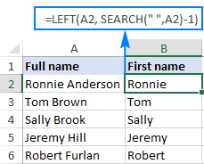
In the same fashion, you can extract the country codes from a column of telephone numbers. The only difference is that you use the Search function to find out the position of the first hyphen ("-") rather than a space:

=LEFT(A2, SEARCH("-", A2)-1)

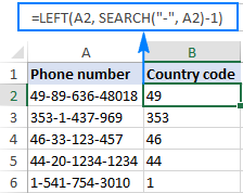
Wrapping up, you can use this generic formula to get a substring that precedes any other character:

How to remove the last N characters from a string

You already know how to use the Excel LEFT function to get a substring from the start of a text string. But sometimes you may want to do something different - remove a certain number of characters from the end of the string and pull the rest of the string into another cell. For this, use the LEFT function in combination with LEN, like this:

The formula works with this logic: the LEN function gets the total number of characters in a string, then you subtract the number of unwanted characters from the total length, and have the LEFT function return the remaining characters.

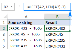
For example, to remove the last 7 characters from text in A2, use this formula:

=LEFT(A2, LEN(A2)-7)

As shown in the screenshot below, the formula successfully cuts off the " - ToDo" postfix (4 letters, a hyphen and 2 spaces) from the text strings in column A.

How to force the LEFT function to return a number

As you already know, the Excel LEFT function always returns text, even when you are pulling a few first digits from a number. What it means to you is that you won't be able to use the results of your Left formulas in calculations or in other Excel functions that operate on numbers.

So, how do you make Excel LEFT to output a number rather than a text string? Simply by wrapping it in the VALUE function, which is designed to convert a string representing a number to a number, like this: VALUE(LEFT())

For example, to extract the first 2 characters from the string in A2 and convert the output into numbers, use this formula:

=VALUE(LEFT(A2,2))

The result will look something similar to this:

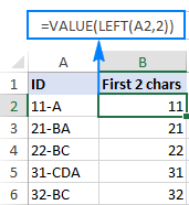
As you can see in the screenshot above, the numbers in column B obtained with a Value Left formula are right-alighted in cells, as opposed to left-aligned text in column A. Since Excel recognizes the output as numbers, you are free to sum and average those values, find the min and max value, and perform any other calculations.

These are just a few of many possible uses of LEFT in Excel. To have a closer look at the formulas discussed in this tutorial, you are welcome to download the Excel LEFT function sample worksheet.

For more Left formula examples, please check out the following resources:

• Split string by comma, colon, slash, dash or other delimiter
• How to split string by line break
• How to convert 8-number to date
• Count the number of characters before or after a given character
• Array formula to perform different calculations on numbers within different ranges

1. Num_chars argument is less than zero

If your Excel Left formula returns the #VALUE! error, the first thing for you to check is the value in the num_chars argument. If it's a negative number, just remove the minus sign and the error will be gone (of course, it's very unlikely that someone will put a negative number there of purpose, but to err is human :)

Most often, the VALUE error occurs when the num_chars argument is represented by another function. In this case, copy that function to another cell or select it in the formula bar and press F9 to see what it equates to. If the value is less than 0, then check the function for errors.

To better illustrate the point, let's take the Left formula we've used in the first example to extract the country phone codes: LEFT(A2, SEARCH("-", A2)-1). As you may remember, the Search function in the num_chars argument calculates the position of the first hyphen in the original string, from which we subtract 1 to remove the hyphen from the final result. If I accidentally replace -1, say, with -11, the formula would through the #VALUE error because the num_chars argument equates to a negative numbers:

2. Leading spaces in the original text

In case your Excel Left formula fails for no obvious reason, check the original values for leading spaces. If you have copied your data from the web or exported from another external source, many such spaces may lurk unnoticed before the text entries, and you will never know they are there until something goes wrong. The following image illustrates the problem:

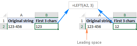
To get rid of the leading spaces in your worksheets, use the Excel TRIM function or the Trim spaces tool.

3. Excel LEFT does not work with dates

If you attempt use the Excel LEFT function to get an individual part of a date (such as day, month or year), in most cases you will only retrieve the first few digits of the number that represents that date. The point is that in Microsoft Excel, all dates are stored as integers representing the number of days since January 1, 1900, which is stored as number 1 (for more information, please see Excel date format). What you see in a cell is just a visual representation of the date and its display can easily be changed by applying a different date format.

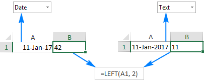
For example, if you have the date 11-Jan-2017 in cell A1 and you try to extract the day by using the formula LEFT(A1,2), the result would be 42, which is the first 2 digits of number 42746 that represents January 11, 2017 in the internal Excel system.

To extract a specific part of a date, use one of the following functions: DAY, MONTH or YEAR.

In case your dates are entered as text strings, the LEFT function will work without a hitch, as shown in the right part of the screenshot: