The tutorial shows how to use the Substring functions in Excel to extract text from a cell, get a substring before or after a specified character, find cells containing part of a string, and more.
Before we start discussing different techniques to manipulate substrings in Excel, let's just take a moment to define the term so that we can begin on the same page. So, what is a substring? Simply, it's part of a text entry. For example, if you type something like "AA-111" in a cell, you'd call it an alphanumeric string, and any part of the string, say "AA", would be a substring.
Although there is no such thing as Substring function in Excel, there exist three Text functions (LEFT, RIGHT, and MID) to extract a substring of a given length. Also, there are FIND and SEARCH functions to get a substring before or after a specific character. And, there are a handful of other functions to perform more complex operations such as extracting numbers from a string, replacing one substring with another, looking up partial text match, etc. Below you will find formula examples to do all this and a lot more.
How to extract substring of a certain length
Microsoft Excel provides three different functions to extract text of a specified length from a cell. Depending on where you want to start extraction, use one of these formulas:
- LEFT function - to extract a substring from the left.
- RIGHT function - to extract text from the right.
- MID function - to extract a substring from the middle of a text string, starting at the point you specify.
As is the case with other formulas, Excel substring functions are best to learn from an example, so let's look at a few ones.
Extract substring from start of string (LEFT)
To extract text from the left of a string, you use the Excel LEFT function:
Where text is the address of the cell containing the source string, and num_chars is the number of characters you want to extract.
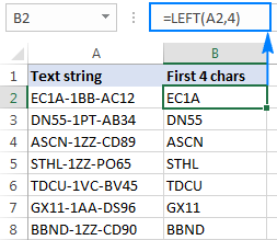
For example, to get the first 4 characters from the beginning of a text string, use this formula:
=LEFT(A2,4)
Get substring from end of string (RIGHT)
To get a substring from the right part of a text string, go with the Excel RIGHT function:
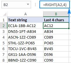
For instance, to get the last 4 characters from the end of a string, use this formula:
=RIGHT(A2,4)
Extract text from middle of string (MID)
If you are looking to extract a substring starting in the middle of a string, at the position you specify, then MID is the function you can rely on.
Compared to the other two Text functions, MID has a slightly different syntax:
Aside from text (the original text string) and num_chars (the number of characters to extract), you also indicate start_num (the starting point).
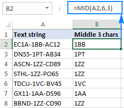
In our sample data set, to get three characters from the middle of a string beginning with the 6th character, you use the following formula:
=MID(A2,6,3)
Tip. The output of the Right, Left and Mid formulas is always text, even when you are extracting a number from a text string. If you want to operate on the result as a number, then wrap your formula in the VALUE function like this:
=VALUE(MID(A2,6,3))
Extract substring before or after a given character
As shown in the above examples, the Left, Right and Mid functions cope nicely with uniform strings. When you are dealing with text strings of variable length, more complex manipulations shall be needed.
Note. In all of the below examples, we will be using the case-insensitive SEARCH function to get the position of a character. If you want a case-sensitive formula, use the FIND function instead.
How to extract text before a specific character
To get a substring preceding a given character, two things are to be done: first, you determine the position of the character of interest, and then you pull all characters before it. More precisely, you use the SEARCH function to find the position of the character, and subtract 1 from the result, because you don't want to include the character itself in the output. And then, you send the returned number directly to the num_chars argument of the LEFT function:
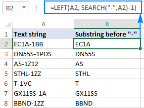
For example, to extract a substring before the hyphen character (-) from cell A2, use this formula:
=LEFT(A2, SEARCH("-",A2)-1)
No matter how many characters your Excel string contains, the formula only extracts text before the first hyphen:
How to extract text after character
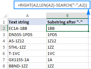
To get text following a specific character, you use a slightly different approach: get the position of the character with either SEARCH or FIND, subtract that number from the total string length returned by the LEN function, and extract that many characters from the end of the string.
In our example, we'd use the following formula to extract a substring after the first hyphen:
=RIGHT(A2,LEN(A2)-SEARCH("-",A2))
How to extract text between two instances of a character
To get a substring between two occurrences of a certain character, use the following generic formula:
The first two arguments of this MID formula are crystal clear:
Text is the cell containing the original text string.
Start_num (starting point) - a simple SEARCH formula returns the position of the desired character, to which you add 1 because you want to start extraction with the next character.
Num_chars (number of chars to extract) is the trickiest part:
- First, you work out the position of the second occurrence of the character by nesting one Search function within another.
- After that, you subtract the position of the 1st occurrence from the position of the 2nd occurrence, and subtract 1 from the result since you don't want to include the delimiter character in the resulting substring.
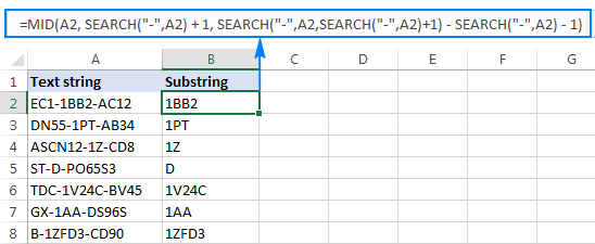
For example, to extract text surrounded by two hyphens, you'd use this formula:
=MID(A2, SEARCH("-",A2) + 1, SEARCH("-",A2,SEARCH("-",A2)+1) - SEARCH("-",A2) - 1)
The screenshot below shows the result:
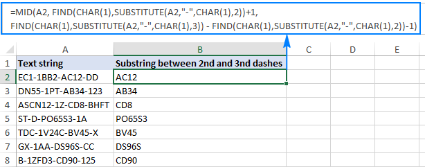
If you are looking to extract text between 2nd and 3rd or 3nd and 4th occurrences of the same character, you can use a more compact SEARCH SUBSTITUTE combination to get the character's position, as explained in How to find Nth occurrence of a character in a string:
In our case, we could extract a substring between the 2nd and 3rd hyphens with the following formula:
=MID(A2, FIND(CHAR(1),SUBSTITUTE(A2,"-",CHAR(1),2))+1, FIND(CHAR(1),SUBSTITUTE(A2,"-",CHAR(1),3)) - FIND(CHAR(1),SUBSTITUTE(A2,"-",CHAR(1),2))-1)
How to find substring in Excel
In situations when you don't want to extract a substring and only want to find cells containing it, you use the SEARCH or FIND function as shown in the above examples, but perform the search within the ISNUMBER function. If a cell contains the substring, the Search function returns the position of the first character, and as long as ISNUMBER gets any number, it returns TRUE. If the substring is not found, the search results in an error, forcing ISNUMBER to return FALSE.
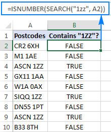
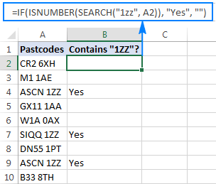
Supposing, you have a list of British postcodes in column A and you want to find those that contain the substring "1ZZ". To have it done, use this formula:
=ISNUMBER(SEARCH("1zz", A2))
The results will look something similar to this:
If you'd like to return your own message instead of the logical values of TRUE and FALSE, nest the above formula into the IF function:
=IF(ISNUMBER(SEARCH("1zz", A2)), "Yes", "")
If a cell contains the substring, the formula returns "Yes", an empty string ("") otherwise:
As you may remember, the Excel SEARCH function is case-insensitive, so you use it when the character case does not matter. To get your formula to distinguish the uppercase and lowercase characters, opt for the case-sensitive FIND function.
For more information on how to find text and numbers in Excel, please see If cell contains formula examples.
How to extract text from cell with Ultimate Suite for Excel
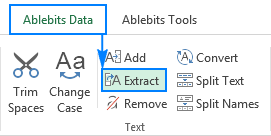
As you have just seen, Microsoft Excel provides an array of different functions to work with text strings. In case you are unsure which function is best suited for your needs, commit the job to our Ultimate Suite for Excel. With these tools in your Excel's arsenal, you just go to Ablebits Data tab > Text group, and click Extract:
Now, you select the source cells, and whatever complex strings they contain, a substring extraction boils down to these two simple actions:
- Specify how many characters you want to get from the start, end or middle of the string; or choose to extract all text before or after a given character.
- Click Insert Results. Done!
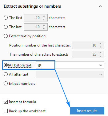
For example, to pull the domain names from the list of email addresses, you select the All after text radio button and type @ in the box next to it. To extract the user names, you select the All before text radio button, as shown in the screenshot below.
And you will get the following results in a moment:

Apart from speed and simplicity, the Extract Text tool has extra value - it will help you learn Excel formulas in general and substring functions in particular. How? By selecting the Insert as formula checkbox at the bottom of the pane, you ensure that the results are output as formulas, not values.
In this example, if you select cells B2 and C2, you will see the following formulas, respectively:
- To extract username:
=IFERROR(LEFT(A2,SEARCH("@",A2)-1),"") - To extract domain:
=IFERROR(RIGHT(A2, LEN(A2)- SEARCH("@",A2) - LEN("@") + 1),"")
How much time would it take you to figure out these formulas on your own? ;)
Since the results are formulas, the extracted substrings will update automatically as soon as any changes are made to the original strings. When new entries are added to your data set, you can copy the formulas to other cells as usual, without having to run the Extract Text tool anew.
If you are curious to try this as well as many other useful features included with Ultimate Suite for Excel, you are welcome to download evaluation version.
More formulas for substrings in Excel
In this tutorial, we have demonstrated some classic Excel formulas to extract text from string. As you understand, there can be almost infinite variations of these basic scenarios. Below you will find a few more formula examples where the Text functions come in handy.
Available downloads
Excel substring functions - practice workbook (.xlsx file)
Ultimate Suite - trial version (.exe file)
 by
by
425 comments
Hi,
Can you please help in excel?
I want to extract the date from a cell and is it possible the word "Date" would be appearing every time just before the date.
I extracted the last 8 characters that contains date (Example of that text --> JSB-EPP-005253-23052022) but the requirement of the format is not achieved. Last 8 characters should be displayed in the assigned cell as "Date: 23.05.2022)".
If this is possible, so please guide me how it would be implemented.
Appreciate your great work,
Thanks & Warm Regards,
Ali
Hi!
To insert characters into text, use the REPLACE function
Try this formula:
="Date: "&REPLACE(REPLACE(RIGHT(A1,8),3,0,"."),6,0,".")
Thank you very very much...this Formula worked great and fulfilled my all requirement :)
I once again appreciate and bundle of thanks Dear Sir..
if I have sentence in one cell, for example :
1. I want to got to "Market"
2. Yesterday, "Old lady" passed away
3. "Car" is expensive
How do you take only the word in between " " sign and copy to other cell (in this case word : Market, Old lady, Car)
Thank you
Hi!
Pay attention to the following paragraph of the article above – How to extract text between two instances of a character. It covers your case completely.
I'm needing to use this for a set of data that sometimes has multiple words in a cell, but not always. I've tried nesting it in an IF formula, but I've gone wrong somewhere. What I have works if there are spaces, but not if there aren't.
Sample data set:
Cat
Brown dog
Mixed-breed dog
I would like to get the following results:
Cat
Brown
Mixed-breed
This formula (where A16 is the original cell) works for the second two, but not the first.
=IF(SEARCH(" ",A16),LEFT(A16,SEARCH(" ",A16)-1),A16)
Hi!
Use the IFERROR function to handle an error when a space is not found.
=IFERROR(IF(SEARCH(" ",A16),LEFT(A16,SEARCH(" ",A16)-1),A16),A16)
That's worked! Thank you!
Hi...!!
I want to check a cell by formula "if a cell contains FORMULA in itself or not".
I am using Excel 2010 so "ISFORMULA" function is not workable for me.
Please advise.
Please advise
Hi
I hope you can help me with this kind sir
In column one, I have a list of tracking numbers that looks like this:
123456
123456
123456
123456
12345678
12345678
12345678
1234567
1234567
12345
12345
12345
Suppose all FedEx trackings are 7 digit numbers, USPS are 8 digits length, DHL are 6 and XPO are the ones with 5 digits.
What I'm trying to do is finding all USPS trackings and extract em from colum 1 to column 2, then, find all FedEx trackings and extract em to column 3, then find all the DHL tracking numbers to column 4 and so on.
Is there a formula for that? Like, one that find all values of a given amount of digits (or characters) in a column and list em in a different column?
Thanks in advance!
(Sorry for the spam, I wasn't sure if I have replied to someone's comment lol)
Hello!
Determine the number of characters using the LEN function. Use the FILTER function to get values of a specific length.
For example:
=FILTER(A1:A20,LEN(A1:A20)=6)
I am looking to extract the text after MA_
RURAL_BUILD_FTTP_28B_FTTP_MA_PCPV9135_ON69848_AGN_SPN_CBT_RURAL_VA1
RURAL_BUILD_28B_FTTP_MA_PCPV9152_POLING_CIVILS_VA1
RURAL BUILD FTTP 30A_FTTP_MA_PCPV9058_MICS_CIVILS_VA1
RURAL BUILD_29A_FTTP_MAIDSTONE_MA_PCPV9027_TEST ROD AND ROPE
Ideally I would like a return of only the V*** after PCP
Any help would be greatly appreciated
Hello!
You can find the examples and detailed instructions here: Extract substring before or after a given character. This should solve your task.
Please How do i extract group of numbers appearing in in different positions of a different cells.
Example;
A
ABSTV234 K:50s
sg789nvhn092h
satcads15qw20
B(outcome)
234
789
15
Hello!
To extract the first number from text string use the user-defined function RegExpExtract. You can find the examples and detailed instructions here: How to extract substrings in Excel using regular expressions (Regex).
"1970000.
00"
how to remove 1st and last 4th char in excel. i excel sheet it is hot showing same.
in excel is display as 1970000.00
i have tried right, left, char, find & replace, int, roundup & etc.
pls help me it is taking lot of time.
Hi!
I am not sure I fully understand what you mean. Explain what result you want to get. Maybe this article will be helpful: How to delete text before or after a certain character in Excel.
Hi Dear,
Can you please help me to extract the text using excel logic
791541213823202211Towage10120
80292721355020228Charts/Publications10.11
80292721355020228Class Certificates / Survey fee (DNV, Lloyd's, GL) / ISM250
80292721355020228Port Costs1897
80292721355020228Port Costs2116.8
80292721355020228Port Costs4.7
80292721355020228Port Costs66.69
80292721355020228Waste Disposal1639.28
90301491169020229Mooring Unmooring1003.89
903643010118Federal Goods and Services Taxes (GST)1633.41
903643010118Federal Goods and Services Taxes (GST)1834.4
903643010118Federal Goods and Services Taxes (GST)2035.4
903643010118Federal Goods and Services Taxes (GST)218.28
903643010118Federal Goods and Services Taxes (GST)230.02
Hello!
To extract everything except numbers from text, you can use the user-defined RegExpExtract function.
=RegExpExtract(A1, "[^\d]+")
You can also find useful information in this article: How to remove numbers from text string in Excel.
Also you can try the formula:
=SUBSTITUTE((CONCAT(IF(NOT(ISNUMBER(--MID(A1,ROW($1:$94),1))), MID(A1,ROW($1:$94),1),"")))," ","")
I hope it’ll be helpful.
Hi All,
not even sure if this is possible. But i need to return the first 5 digit number from the below alphanumeric text in a cell. the answers should be
Example 1: 93423
Example 2: 87952
Example 1: "**02.06 return updated in SPA** ordered 93423 BR 4PNS PCFC A RK 495L 1X1 x 2 delivered 2 x 4Pns Pl Al 94253 1300353110"
Example 2: noted with d Short delivered multiple invoices - 2 x BR Vct Br NGB 750 4x3 87952 12 x BR PI N A 5.1% NGB 330ML 4X6IMP 94152
Hello!
You can solve your problem with a user-defined REGEX function. The following tutorial should help: How to extract substrings in Excel using regular expressions (Regex). To extract a five digit number, try this formula:
=RegExpExtract(A1, "\d{5}", 1)
1. Having input with total four remarks “Received, waived, OTC due, PDD due”
a. In Column “A" I have number of documents with document description
b. In Column “B" I have dropdown of Copy or Original
c. In Column “C" I have Remark of "Received" for Respective document
d. In Column “E" I have Remark of "Waived" for Respective document
e. In Column “F" I have Remark of "Short due" for Respective document
f. In Column “G" I have Remark of " Long due" for Respective document
2. Outcome required
a. In Column “A" I required document description either in copy or original having remarks “Received” (1st scenario)
b. In Column “A" I required document description either in copy or original having remarks “Short due & Long due” (2nd scenario)
c. In Column “B” I required document nature with outcome of copy or Original as per input data (Required in both scenario)
Please help here to extract the outcome it will be great help for me thanks in advance
Hi!
I am not sure I fully understand what you mean. You want to put the result in column A, which already has data. Please provide me with an example of the source data and the expected result.
Point no 1 Narrate about it's source data through subhead which was inputted in sheet no 1
& point no 2 narrate about required outcome through source data in sheet no 2 therefor I mention column A & B in both Point because these refer two different sheet. I mention the sample data below for sheet 1. please update excel formula which i can use in sheet 2 of same excel.
DOCUMENT TYPE Received Waived Short due Long due
sale deed Copy Received
RD Copy Waived
Death certificate Copy Waived
sale deed 2 Copy Received
ATS Original Short due
SPA Original Short due
sale deed Original Long due
RD Original Long due
Death certificate Original Long due
Due to some limitation unable to paste excel sheet therefor i mention revised source data for sheet one plz copy & paste the data in excel sheet & share the formula in sheet two
a. In Column “A" of sheet 1
DOCUMENT (Heading)
sale deed
RD
Death certificate
sale deed 2
ATS
SPA
sale deed
RD
Death certificate
b. In Column “B" of sheet 1
TYPE (Heading)
Copy
Copy
Copy
Copy
Original
Original
Original
Original
Original
c. In Column “C" of sheet 1
RECEIVED (Heading)
Received
BLANK
BLANK
Received
BLANK
BLANK
BLANK
BLANK
BLANK
d. In Column “E" of sheet 1
WAIVED (Heading)
BLANK
Waived
Waived
BLANK
BLANK
BLANK
BLANK
BLANK
BLANK
e. In Column “F" of sheet 1
SHORT DUE (Heading)
BLANK
BLANK
BLANK
BLANK
Short due
Short due
BLANK
BLANK
BLANK
f. In Column “G" of sheet 1
LONG DUE (Heading)
BLANK
BLANK
BLANK
BLANK
BLANK
BLANK
Long due
Long due
Long due
Outcome required in sheet 2
1. In Column “A" of sheet 2
a. I required document description either in copy or original having remarks “Received” (1st scenario)
b. I required document description either in copy or original having remarks “Short due & Long due” (2nd scenario)
2. In Column “B" of sheet 2
c. I required document nature with outcome of copy or Original as per input data (Required in both scenario)
Hi!
I’m not sure I got you right since the description you provided is not entirely clear. However, it seems to me that FILTER function will work for you.
You can find the examples and detailed instructions here: Excel FILTER function - dynamic filtering with formulas.
hey
i have a data i need to do the following
1- i need to select the word ( black )
2- i need to delet it from the A1 cell
3- i need to replasce it in cell b1
ex.
A1 iphone 6s black
A2 iphone black 7p
A3 black flat charger
what i want to do is
A1 iphone 6s B1 black
A2 iphone 7p B2 black
A3 flat charger B3 Black
thank you
Hi!
If I understand your task correctly, the following tutorial should help: Using REPLACE and SUBSTITUTE functions in Excel.
Excellent content as usual
xboxonefifa14
3dspokemonmoon
playstation3ufcundisputed3
playstation3djhero
playstation3fifa14
xbox360pure
xboxoneforzahorizon2
playstation2needforspeedunderground
playstation4yakuza0
xbox360worms2armageddon
playstation4soulcaliburvi
xboxonehitman2
Hello, I am looking for a way to split the game platforms; (xbox360, xboxone, playstation2, playstation3, 3ds etc) from the game titels; (fifa14, pokemonmoon, djhero etc). Is there a formula I could use ? I tried this formule: =IF(SEARCH("one";A2;2);LEFT(A2;SEARCH("one";A2)+2);1) to split xboxonefifa14 which only worked to split xboxone from the game title, but I couldn't get the game title in a different column. So my question is how I could be able to separate the game titles from different platforms?
Hello!
To get the name of the game in the second column, use the SEARCH function to find the game platform. Replace game platform with blank using the SUBSTITUTE function.
=CONCAT(IF(ISNUMBER(SEARCH($H$1:$H$5,A1)), SUBSTITUTE(A1,$H$1:$H$5,""),""))
$H$1:$H$5 - game platforms.
You can also find useful information in this article: How to find and replace multiple values at once.
Hi,
Thanks for the reply! The formula worked for the most games and I managed to separate the games from the game platform. However, I do run into trouble with the game platforms; xboxone, xbox360, xboxseriesx, pc and 3ds.
xboxonefifa14 fifa14onefifa14
3dspokemonmoon pokemonmoon3pokemonmoon
playstation3ufcundisputed3 ufcundisputed3
playstation3djhero djhero
playstation3fifa14 fifa14
xbox360pure pure360pure
xboxoneforzahorizon2 forzahorizon2oneforzahorizon2
playstation2needforspeedunderground needforspeedunderground
playstation4yakuza0 yakuza0
xbox360worms2armageddon worms2armageddon360worms2armageddon
playstation4soulcaliburvi soulcaliburvi
xboxonehitman2 hitman2onehitman2
playstation3nhl13 nhl13
xboxseriesxassassinscreedvalhalla assassinscreedvalhallaseriesxassassinscreedvalhalla
pctransistor transistor
pclifeisstrange2episode3wastelands pclifeisstrange2episode3wastelanlifeisstrange2episode3wastelands
These are a few games I tried to seperate. Do you have any idea what might cause this problem and why it doesn't replace the game platform with a blank value and copies the game + gameplatform instead?
The formula I used: =CONCAT(IF(ISNUMBER(SEARCH($H$2:$H$21;A2)); SUBSTITUTE(A2;$H$2:$H$21;"");""))
Input for H:
xboxone
xbox360
playstation3
playstation4
playstation2
playstationvita
playstation5
wii
switch
3ds
psp
ds
gameboyadvance
dreamcast
xboxseriesx
xbox
gamecube
pc
wiiu
stadia
Hi!
The names of the gaming platforms have partial matches. If you search for xbox360 it will find xbox360 and xbox. Also "ps" can be found in the name of the game.
FI_AC_BONDS
FI_AC_OBU_LIQ
FI_AC_SUKUK
FI_AC_SUK_OBU
FI_AFS_BONDS
FI_AFS_OTH_BUS
FI_AFS_ST
FI_AFS_SUKUK
FI_AFS_SUK_OBU
UNB_FI_AFS_BOND
UNB_FI_AFS_SUK
I want to find if AFS or AC word is available on above table and need to get in displace as AFS or AC in another cell.
Hi!
Based on your description, it is hard to completely understand your task. However, I’ll try to guess and offer you the following formula with SEARCH function:
=IF(ISNUMBER(SEARCH("AFC",A1)),"AFC",IF(ISNUMBER(SEARCH("AC",A1)),"AC",""))
If this is not what you wanted, please describe the problem in more detail.
Cell A1 contains Iim Rd, Near Kendriya Vidyalaya, Mubarakpur, Lucknow, Uttar Pradesh 226201
Cell A2 contains Lucknow
I need to extract until Lucknow into Cell A3 using a Formula
Cell A3 FINAL VALUE should be Iim Rd, Near Kendriya Vidyalaya, Mubarakpur ( with or without comma ) is ok
Hi!
Pay attention to the following paragraph of the article above - How to extract text before a specific character.
It covers your case completely.
Hello!
thanks for this very interesting article. Can you help me to solve this problem
[{ 12, name: Adventure}, { 14, name: Fantasy}, { 28, name: Action}]
i wana making colum B Adventure; colum C Fantasy and Colum C Action
Rin (Re.1) Advanced Detergent Powder, 10g (Pack of 108) (IA) = 108
Lays (Rs.10) Potato Chips - Cream & Onion, 30g (Pack of 10) (IA) = 10
Parachute (Re.1) 100% Pure Coconut Hair Oil, 2.3ml (Pack of 36) (IA) =36
Too Yumm! (Rs.5) Veggie Stix - Chilli Chatka, 14g (Pack of 12) (IA) =12
Please help here to extract the number after the word " Pack of"
Hello!
I believe the following formula will help you solve your task:
=IFERROR(MID(A2, SEARCH("Pack of ", A2) + LEN("Pack of "), SEARCH(") (", A2) - SEARCH("Pack of ", A2) - LEN("Pack of ")), "")
Read more in this article: How to extract text between two characters or words.
No sir,
Its not working ,
showing blank when i apply this formula.
Hi!
I tested the formula using your data. She works.
Hello Sir
The given formula not working for below cases,
1.Pampers Baby Dry Pants - M, 2pcs, (Pack of 8)
2.Colgate (Rs.10) Active Salt Toothpaste, 21g (Pack of 12)
Hi!
The formula I sent to you was created based on the description you provided in your first request. However, as far as I can see from your second comment, your task is now different from the original one. For this data, another formula is needed.
=IFERROR(MID(A2, SEARCH("Pack of ", A2) + LEN("Pack of "), SEARCH(")",A2,SEARCH("Pack of ", A2)+1)- SEARCH("Pack of ", A2) - LEN("Pack of ")), "")
Supper Sir,
Great Thanks.....
I am trying to extract the month from a string like the following
CF Customer Oct 07
Ash Customer Sep 07
Pete Customer Sep 07
Can you give me a formula?
Hello!
To extract a string from text, try using the MID function -
=MID(A1,LEN(A1)-5,3)
Hope this is what you need.
Hi,
Can you please suggest in this, will appreciate your help.
I have some cells like below
Sushama.K.CTS -> Sushama.K.CTS -> Arbina.B.CTS
Snehal.C.CTS -> Pooja.G.CTS
Sonam.C.CTS -> Sonam.C.CTS -> Sonam.C.CTS
Sonali.S.CTS -> Sonali.S.CTS -> Sonali.S.CTS -> Sonali.S.CTS -> Sonali.S.CTS
How I can extract the last name from each cells after the ">" symbol.
Like, my result for above cells should be like
Arbina.B.CTS
Pooja.G.CTS
Sonam.C.CTS
Sonali.S.CTS
I have tried with this formula,
=RIGHT(Q3424,LEN(Q3424)-SEARCH(">",Q3424))
but it's giving me this result
Sushama.K.CTS -> Arbina.B.CTS
Pooja.G.CTS
Sonam.C.CTS -> Sonam.C.CTS
Sonali.S.CTS -> Sonali.S.CTS -> Sonali.S.CTS -> Sonali.S.CTS
but I need the last part
So please suggest.
Hello!
Replace the last ">" with "#" using the SUBSTITUTE function. Determine the position of this character using the SEARCH function. Starting from this position, extract string from the text using the MID function.
=MID(SUBSTITUTE(A1,">","#",LEN(A1)-LEN(SUBSTITUTE(A1,">",""))), SEARCH("#",SUBSTITUTE(A1,">","#",LEN(A1)-LEN(SUBSTITUTE(A1,">",""))))+1,50)
This should solve your task.
Hi, I have a query , it would be great if you could solve this. I have some UPC codes in one cell, i need to copy all the UPC codes into different excel cells.
077346100626, 011951600003, 781968002106, 692000196342, 885694471981, 715933319937, 199960027704
I need to copy numbers after every "," sign to different cells.
Like
077346100626
011951600003
781968002106
692000196342
885694471981
715933319937
199960027704
Thanks,
Hello!
We have a special tutorial on this. Please see How to split text string in Excel by comma, space, character or mask.
its helpful, but it didn't solve my problem. In the tutorial which you told me, it find the characters in a three word cell, but in my case i have more than 5 or more words separated by ","
How can i separate them by this formula ?
in the tutorial it used three functions 1-Left 2-Mid 3-Right
Is there any thing else i can use to solve this problem ?
Hello!
You can use the Split Text tool included with our Ultimate Suite for Excel that you can install in a trial mode and check how it works for free.
Try to use the recommendations described in this article: How to split cells in Excel.
Hope you’ll find this information helpful.
Pozdrav !
Kako izvuci jednu rec iz jedne celije u kojoj ima vise reci ? Evo nekoliko primera celija iz kojih treba izvuci odredjene reci :
H1 BRENT_OIL at 02:55:02 SuperTrend up -(jedna celija)
3_Level_ZZ_Semafor_NRP Alert on CrudeOIL, period M15: SELL SIGNAL Level2 -(jedna celija)
Apollo Scalper CADCHF M15 BUY @0.74719, TP 0.75019, SL 0.74569 -(jedna celija)
Problemi : Jedna trazena rec ima vise znacenja : (UP,BULISCH,BUY) Drugi primer : (SELL,BEARISH,DOWN).
Trazena rec nije uvek na istom mestu u celiji. Kako postaviti formulu koja jednostavno pita prvu celiju da li se u njoj pojavila jdna trazena rec : (UP,BULISCH,BUY) ili (SELL,BEARISH,DOWN) Postavio bih formulu za prvo pitanje u recimo D2 a za drugo E2. Ako se bilo koja rec od trazenih pojavi moze se napisati u istoj celiji gde je postavljena formula ili nekoj drugoj svejedno... Tako bih sa te dve kolone pratio signale koji se pojavljuju u prvoj koloni ? Svasta sam probao pa sam se zamrsio izgleda jednostavno ali je zapetljano...Primeri koje sam koristio pa mi nije bas sve uspelo :
=IF(SEARCH("UP",D2),G10,H10) =IF(ISNUMBER(SEARCH("UP",D2)),G10,H10)
=IF(SUMPRODUCT(-ISNUMBER(SEARCH("UP",D2:D2))),"0","UP") =TRIM(MID(D2,SEARCH("UP",D2)+10,LEN(D2)))
=IF(ISNUMBER(SEARCH("supertrend",D2)),G2,"")&IF(ISNUMBER(SEARCH("apollo scalper",D2)),G3,"")
Itd... Hvala
Goran
Hello!
How to extract one word from one cell that contains several words? Here are some examples of cells from which certain words are extracted:
H1 BRENT_OIL at 02:55:02 SuperTrend up - (single cell)
3_Level_ZZ_Semaphore_NRP CrudeOIL warning, period M15: SALES SIGNAL Level 2 - (single cell)
Apollo Scalper CADCHF M15 BUY @ 0,74719, TP 0,75019, SL 0,74569 - (single cell)
Problems: One search word has several meanings: (UP, BULISCH, BUY) Another example: (SELL, BEAR, DOWN).
The search word is not always in the same place in the cell. How to set up a formula that simply asks the first cell if one of the search words appeared in it: (UP, BULISCH, BUY) or (SELL, BETTER, DOWN) I would set the formula for the first question in say D2 and for the second E2. If any of the words of the requested occurrence can be entered in the same cell where the formula is located or someone else doesn't care ... So, I would follow the signals that appear in the first column from those two columns? I tried everything, so I was confused, it looks simple, but it's complicated ... Examples I used, so I didn't succeed:
= IF (SEARCH ("UP", D2), G10, H10) = IF (NUMBER (SEARCH ("UP", D2)), G10, H10)
= IF (SUMPRODUCT (-UM (SEARCH ("UP", D2: D2))), "0", "UP") = TRIM (CENTER (D2, SEARCH ("UP", D2)) + 10, LEN D2)))
= IF (ISBROJ (SEARCH ("supertrend", D2)), G2, "") & IF (ISBROJ (SEARCH ("apollo scalper", D2)), G3, "")
Etc ... Thanks
Goran
Hello!
If I understand the problem correctly, you can use the SEARCH function to search for the desired word. With nested IF functions, you can check two conditions.
Please try the formula below:
=IF(SUM(--ISNUMBER(SEARCH({"UP","BULISCH","BUY"},A2))) > 0,$D$2, IF(SUM(--ISNUMBER(SEARCH({"SELL","BEARISH","DOWN"},A2))) > 0,$E$2,""))
I hope it’ll be helpful. If something is still unclear, please feel free to ask.
Pozdrav !
OK Pomaze Thanks
Goran
Super helpful. Thanks
Hello Alexander,
I hope you can help me, I have a list of transactions in column J and a list of text in a separate tab in the same workbook. I want to write a formula to find this text in the separate tab and extract this from the transactions (Column J) and the result should be in Column N.
For Example:
Column J
"Int Debit Order To Settlement
"Cashsend Digital SettlementCard No.
Digital Tran Fees Settlement *
Bal Brought Forward
Monthly Acc Fee Headoffice *
Transaction Charge Headoffice *
"Int Debit Order To Settlement"
"Acb Debit:External Settlement 19.75 "
"Digital Transf Cr Settlement"
"Atm Withdrawal 31.50 TCard No. "
"Pos Purchase Settlement 4.35 TCard No. (Effective 16/05/2022)"
"Notific Fee Sms Notifyme 1.20 T2 Sms Notifications"
PY 4654654654Transfer
Separate Tab List in Column Q:
Notific Fee Sms
Bal Brought Forward
Pos Purchase
Acb Debit:External
Transaction Charge
Monthly Acc Fee
Cashsend Digital
PY 4654654654
Int Debit Order To
Digital Tran Fees
Atm Withdrawal
In Column N:
I need the formula to search from the list (Separate Tab) and extract the text from the transactions in Column J.
If you could assist me with this formula please.
Hello!
To search for a string in text, use the SEARCH function.
Use INDEX+MATCH to get the desired values.
Please try the following formula:
=INDEX(J1:J13,MATCH(TRUE,ISNUMBER(SEARCH(Q1,J1:J13)),0))
Hope this is what you need.
Hi
Please resolve my below problem:
I Have data in cells as below:
A1= 1B90
A2= 1B113
A3= 3DE- 61
A4= 1E-105
And I want as below:
B1= B
B2= B
B3= DE
B4= E
Hello!
To extract only letters from text, use regular expressions.
Try to use the recommendations described in this article: How to extract substrings in Excel using regular expressions (Regex).
=CONCAT(RegExpExtract(A1;"[a-zA-Z]+"))
I hope my advice will help you solve your task.
Hi
I need to extract whatever string is between the 3rd and 4th undercover of the texts below:
asd_KSA_Consideration_LocalFootball_Beverages_Core 18-34_Trueview_Youtube_CLE_February2022_1546960|1862997
Here the answer should be "LocalFootball"
asd_KSA_Awareness_LocalFootball_Beverages_Core 18-34_Bumper Ads_Youtube_CLE_February2022_1546960|1440241
Here the answer should be "LocalFootball"
asd_KSA_Awareness_LaunchKSA_Beverages_CoreAudience_Bumper Ads_Youtube_CLE_BLS_March2022_1918871|1311320
Here the answer should be "LaunchKSA"
asd_KSA_Consideration_LaunchKSA_Beverages_InMarket_Discovery Ads_Youtube_CLE_BLS_February2022_1918871|1740112
Here the answer should be "LaunchKSA"
asd_KSA_Awareness_LaunchKSA_Beverages_CoreAudience_Video_DV360_PGD_Adintop_February2022_1918871|1014779
Here the answer should be "LaunchKSA"
asd_KSA_Conversion_LaunchKSA_Beverages_CoreAudience_Video_DV360_PGD_DMS_February2022_1918871|1883124
Here the answer should be "LaunchKSA"
asd_KSA_Consideration_LaunchKSA_Beverages_CoreAudience_Trueview_Youtube_CLE_BLS_February2022_1918871|1362081
Here the answer should be "LaunchKSA"
asd_KSA_Conversion_Launch_Beverages_CoreAudience_Video_DV360_PGD_Vidmatic_March2022
Here the answer should be "Launch"
asd_KSA_Conversion_Launch_Beverages_CoreAudience_Video_DV360_PGD_Vidmatic_March2022_Cancelled
Here the answer should be "Launch"
asd_JOR_Consideration_Max_Beverages_Core 18-35_Trueview_Youtube_CLE_March2022_OD22|3228
Here the answer should be "Max"
asd_JOR_Awareness_Max_Beverages_Core 18-35_Bumper Ads_Youtube_CLE_March2022_OD22|3228
Here the answer should be "Max"
asd_KSA_Awareness_CFBQ1_Beverages_CoreAudience_Video_DV360_PGD_MMP_February2022_1963621|1373446
Here the answer should be "CFBQ1"
asd_KSA_Awareness_CFBQ1_Beverages_CoreAudience_Video_DV360_PGD_DMS_February2022_1963621|1564216
Here the answer should be "CFBQ1"
asd_KSA_Consideration_CFBQ1_Beverages_CoreAudience_Trueview_Youtube_CLE_BLS_February2022_1963621|1508651
Here the answer should be "CFBQ1"
Hello!
The following tutorial should help: How to extract Nth word from text string.
I hope I answered your question. If something is still unclear, please feel free to ask.
Hello,
I have the following statement where I'm trying to pull the numerical value's off the far right side (a: 157.00; b: -0.23; c: 9.00). I have tried the example up the top for RIGHT function but it jut pulls everything excluding the month (Feb). If I drop the LEN function and just use SEARCH it pulls only four characters from the right (a:7.00; b:0.23; c: 9.00).
Feb 07 Mudgee Vet Surg Mudgee Au 034254325786123489 157.00
Feb 06 Temple & Webster St Peters Au 25643965992308034556 -0.23
Feb 05 The Brumby Nepalese R Nadal Au 75123502038260262235719 9.00
Thank you for your help in advance.
Cheers,
Rowie
Hello!
Look for the example formulas here: How to extract number from the end of text string.
This should solve your task.
Dear Sir,
I have texts in a large xls in the pattern of
APLHA|Alphanum1|alpha num2|alpha num3 - the length of each alphanum is not fixed. Text has spaces too.
I need to get all the text upto the last | delimiter - i.e. - "APLHA|Alphanum1|alpha num2"
Could not make any of the above work. Please assist.
Hello!
Use the SUBSTITUTE function to replace the last delimiter with another character. Calculate the position of this character using the SEARCH function. Get the required number of characters using the LEFT function.
=LEFT(A1,SEARCH("#",SUBSTITUTE(A1,"|","#", LEN(A1)-LEN(SUBSTITUTE(A1,"|",""))))-1)
I hope my advice will help you solve your task.
Primary Street Stored in A1
560, 95, Kanpur Road, Krishna Nagar Village, Krishna Nagar, Alambagh, Lucknow, Uttar Pradesh 226023
Primary City Lucknow Stored in A2
a3 should retun text to left of Lucknow ( a2 )
ie., 560, 95, Kanpur Road, Krishna Nagar Village, Krishna Nagar, Alambagh,
Thanks in advance
Hi!
Use the SEARCH function to determine how many characters are to the left of the Primary City.
Extract the required number of characters with the LEFT function.
=LEFT(A1,SEARCH(A2,A1)-1)
I hope my advice will help you solve your task.
Thanks Brother, it helped
I need to find the string before "-DT" or "-LT" from following
QDY3-DT-HC00121
ZYN-LT-000013
CN-URB-LT-00036A23
WILT-DT-LPD001
so the results would looks as follows
QDY3
ZYN
CN-URB
WILT
Hi!
Pay attention to the following paragraph of the article above: How to extract text before a specific character.
It covers your case completely.
=LEFT(A2, IF(ISNUMBER(SEARCH("-DT",A2)-1),SEARCH("-DT",A2)-1,SEARCH("-LT",A2)-1))
To use two search conditions, use a nested IF function.
Thanks for the response, it works perfectly. also I referred the above mentioned paragraph but still couldn't understand logic being used in this formula :( . would you be able to explain your formula. also if I want to add one more string "-SRV", what would be the new formula. hope that would help me to understand the logic
Hi!
To search for multiple variants of a specific character, you can use the formula
=CONCAT(IFERROR(LEFT(A2,SEARCH({"-SRV","-DT","-LT"},A2)-1),""))
The IFERROR function will replace failed search errors with empty strings. The CONCAT function converts an array of search results into a single text string.
Hello
if i cells with:
111222
11222
1222
and i want extract "1" from them like this:
111
11
1
how i can do it?
Hello!
Use substring functions to extract text from cell:
=LEFT(A1,SEARCH(2,A1)-1)
Hope this is what you need.
Hi can you kindly help me, i have a situation where in a cell there is a few items that i need to separate out into different columns
"Item 1. D/W RSC (CTN 35)
Material Code: -
Quantity: 1,000 piece
Account Name (GL): OPS PACKING MATERIALS (4340000)
BusA/CC: AM71/AM2D
Mandatory to Quote: Yes
Item 2. D/W CTN (CTN 90)
Material Code: -
Quantity: 1,000 piece
Account Name (GL): OPS PACKING MATERIALS (4340000)
BusA/CC: AM71/AM2D
Mandatory to Quote: Yes
Item 3. D/W CTN (CTN 98)
Material Code: -
Quantity: 2,000 piece
Account Name (GL): OPS PACKING MATERIALS (4340000)
BusA/CC: AM71/AM2D
Mandatory to Quote: Yes
Item 4. D/W RSC (CTN 56)
Material Code: -
Quantity: 1,000 piece
Account Name (GL): OPS PACKING MATERIALS (4340000)
BusA/CC: AM71/AM2D
Mandatory to Quote: Yes
Item 5. S/W RSC (CTN 28)
Material Code: -
Quantity: 1,000 piece
Account Name (GL): OPS PACKING MATERIALS (4340000)
BusA/CC: AM71/AM2D
Mandatory to Quote: Yes
( This is all in 1 cell)
How do I separate them
I'm in desperate need, please help me, thank you
Hello!
If you want to split text into cells by line break, you can use the Excel tool - Text to columns. Use the key combination CTRL+J to specify line feed as "other" character.
You can also use the Split Text tool. It provides many options to split text into cells. It is available as a part of our Ultimate Suite for Excel that you can install in a trial mode and check how it works for free.
is there any formulas that i can use?
Hello!
we have columns of data in each - mention below.
Please help us to segregate M followed by 8 digits in a separate cell.
-------------------------------------------------------------
"3 laptops
Po# m17121848 item # 9999207718877
Po# m18147289 item # 9999207707199
Po# m34283154 item # 9999207718875"
-------------------------------------------------------------
"p.o m31153508
item number 9999207495586"
-------------------------------------------------------------
"p.o. m355515737
item number 9999207564615"
-------------------------------------------------------------
"p.o m31153508
item number 9999207495586"
------------------------------------------------------------
"p.o m31153508
item number 9999207495586"
-------------------------------------------------------------
Hello!
To extract part of the text from a string, use the MID function:
=MID(A2,SEARCH("m",A2),9)
I hope it’ll be helpful.
Thanks for the response. The above formula is working for Single M in single cell but we have more of multiple M************** in single excel cell. can you please us to provide mulitple M formula.
For example:
Below data available in single excel cell.
Po# m17121848 item # 9999207718877
m18147289 item # 9999207707199
Pom34283154 item # 9999207718875"
Hi!
Specify exactly what results from your data you want to get.
i want to get M followed by 8 digit. i have multiple occurrence Mxxxxxxx in a single cell data. on this formula (=MID(A2,SEARCH("m",A2),9)) work for single occurrence of M followed by 8 digits please help me to get all other occurrence of M.
we want to extract multiple occurrence of M with 8 digits only in single cell data. for example
we have data in a single cell of below
Po# m17121848 item # 9999207718877
m18147289 item # 9999207707199
Pom34283154 item # 9999207718875"
we want to get in a cell like below:
M17121848
M18147289
M34283154
Thanks for your help.
Hi!
Use regular expressions to solve your problem.
Use a custom function RegExpExtract:
=RegExpExtract(A1,"m\d+")
You can find the examples and detailed instructions here: How to extract substrings in Excel using regular expressions (Regex).
I hope I answered your question. If something is still unclear, please feel free to ask.
Hi,
I have this data and I need to extract only the characters under the format M9xxxxxxxxxx.
M90000000001; 1062172; 4503260578
M90000000002; L20000000001; M90000000005
M90000000003
I am using the formula: =MID(A2,FIND("M9",A2,1),12) but this does not bring all the data, in case I have 2 values in a single cell M9xxxxxxxxxx (i.e. line 2).
Is there a way to extract both?
Thank you!
Hello!
Separate your long text values into individual cells using semicolons as delimiters. See detailed instructions here: How to split cells in Excel: Text to Columns, Flash Fill and formulas.
After that, you can use your formula.
Thank you for the suggestion!
Hello!
I have data in this format under excel sheet.
I only want to extract characters from the below column, how do I leave/remove special characters (unwanted symbols) and only extract characters which are present in each row.
Please help me..
location
Yakima, WA
Distrito Federal, México
Prison
?
laugh of january
Karachi, Pakistan
kiwook. ♡
grace, she/her, 24
QATAR
eve ♡ [swe/eng/한]
Bengaluru, India
Saudi Arabia .Taif
kiwook. ♡
Lab of Womb
Nederland
Calabria, Italia
Iraq
Alexandria/Tanta
#everywhere
Ruwa Zimbabwe
Reality
Ayodhya
Maldives
??
Szczecin, Polska
Hargeisa, Somaliland
Prosthodontics Section, CoD
Davao City, Davao Region
under these bitches’ skin
Islamabad, Pakistan
??
khandwa mp
New York, NY ✈️ Houston, TX
United Arab Emirates
Atlantis
Lampung, Indonesia
08/30/17
Jakarta Pusat, DKI Jakarta
losers club
tyler williams inc
Kharkhoda, India
Iraq
Tweets are my own and not representative of my employer
Philippines
Jeddah - khartoum
Madinah
Hello!
To remove special characters from text, you can use regular expressions. You can find the examples and detailed instructions here: Excel Regex to remove certain characters or text from strings.
You can use this formula:
=TRIM(RegExpReplace(A5, "[^0-9a-zA-Z\.,/ ]+", ""))
You can also use Regex Tools for Excel. With Regex Tools, which are part of Ultimate Suite for Excel, you can find, extract, remove, or replace strings that match a pattern.
Hello, I have a task to extract a specific location code from a string. Examples from the text I am using are as follows:
AUS177-4M
Canada551-3W
MEX316-3W
US160-3Mo
ARG265-2W
MEX363-5Mo
US351-4W
GER195-6Mo
GER529-2Mo
AUS301-7Mo
GER60-3W
ENG102-8Mo
AUS219-9W
ENG342-10Mo
US476-11M
GER93-6W
GER442-10M
Japan17-8W
Canada559-11Mo
ARG389-11Mo
Canada121-12M
As you can see the data aren't neatly arranged, nor are they all a set amount of characters long. I need to be able to extract the location text (Canada, GER, US, Japan) exactly as it appears in the text string and display it in another column. Is there any way you could assist me in this?
Hello!
To extract all characters up to the first digit in the text, try using the formula
=LEFT(A2,MIN(IF(ISERROR(FIND({1;2;3;4;5;6;7;8;9;0},A2)), "",FIND({1;2;3;4;5;6;7;8;9;0},A2)))-1)
Hope this is what you need.
If I just wanted to display the number or letter(s) at the end of a string, would this approach work also? For example, If I had HSM-11Mo, and I wanted to display just the 11 or the Mo inside of a column by itself, would I be able to with this type of formula? I am not an excel expert by any means so I apologize for any confusion in my statement.
Hello!
If you want to show all characters after the last digit, then try this formula:
=MID(A2,LOOKUP(,-MID(A2,ROW($1:$99),1),ROW($1:$99))+1,50)
This formula works on most of the cells in my data set but a few of them still include the dash and number. For example, the data
NGE270-18M
SUA110-5M
EXM390-18Mo
NGE430-17W
would all return a -18M or -18Mo or -17W depending on the cell. Is there anyway I can fix this?
Hi!
Read carefully this paragraph and the example above: How to extract text after character.
This is the answer to your question.
I have data in this format under excel sheet.
S02E01.the.Wild.Goose.Chase
S02E02.Needle.in.a.Haystack
S02E03.Might.of.the.Atwal.Empire
S02E04.True.Lies
S02E05.Wedding.Bells.Make.a.Loud.Sound
S02E06.Revenge.Is.Best.Served.Cold
S02E07.the.Girl.and.the.Cop
S02E08.Goons.Guns.and.Bombs
S02E09.the.Hunter.Is.Now.the.Hunted
S02E10.Thats.the.Way.the.Cookie.Crumbles
I want result as any data excluding starting 7 characters.
Thanks
Hello!
To extract a portion of text starting at a specific position, use the MID function -
=MID(A1,8,50)
Hello
I would appreciate any help. I have a high volume of the below data (located in one cell);
"Winning Combination: 2/1/1/1/1/2/1/1/3/1
Status: Official
Results: (9/10)
Winners: 2015.43
Dividend: R42.60
Results: (10/10)
Winners: 141.00
Dividend: R2,439.80"
I need to extract;
2015.43
42.60
141
2439.80
Any advice?
Thanks
Hello!
To extract numbers from text, you can use regular expressions. You can find detailed instructions and examples in this article: How to extract substrings in Excel using regular expressions (Regex).
Hi there. I have a column with notes where I want to extract the 15 digits that appear after IRCT (or irct), including the IRCT into an adjacent (blank) column. The IRCT number can appear anywhere in the cell.
E.g. (2022-02-09 16:24:37)(Select): irct2012042495523N1;
or IRCT2017011520145N4; (2021-09-01 15:31:36)(Screen): #66 Abdollahi 2019 might be linked & has abstract
Are you able to help? I can only find instructions for extracting a) after a single character (not a string) and no instructions for specifying the length of the string to be extracted.
Thank you!!
Hello!
Please use the following formula -
=MID(A1,SEARCH("irct",A1),19)
The article above has all the information you need. I hope it’ll be helpful.
Thank you for this!! I was looking for something similar.
Brilliant! Thank you so much for the quick response - much appreciated :-). One final question, if the cell doesn't contain "irct", what is the argument for returning a 0, rather than #VALUE!)
Hello!
To replace an error message with a value, use the IFERROR function.
You can use this formula:
=IFERROR(MID(A1,SEARCH("irct",A1),19),0)
How Can I select sugar and flax from this formula
"Milk, sugar, Vegetable shortening, canola oil, milk powder, cardamom essence, whole wheat flour, flax seed, raisin, sugar, almond, cashew"
what formular can i use to extract only characters in a cell without the LAST 4 DIGITS
e.g "Vitamin A supplementation 6-11 months 2019" results should be "Vitamin A supplementation 6-11 months"
and
"LLIN given to pregnant women 2021" results should be "LLIN given to pregnant women"
Hello!
Extract all characters from the text, except the last four. Use the LEFT and LEN functions.
=LEFT(A1,LEN(A1)-4)
I hope I answered your question.
it worked!!, thanks
Hi,
I have cells containing this pattern:
A.BBBBB
A.B.CCCCCCC
A.B.C.DD
How do I get the substring to the right of the utmost right period, e.g. BBBBB, CCCCCCC, DD?
TIA!
Hello!
To extract the text at the end of a string, use regular expressions as described in this tutorial: How to extract substrings in Excel using regular expressions (Regex).
Pattern: \w+$
This should solve your task.
Thanks Alexander, this helps a lot, though not completely, since some of the strings look like A.B.C.DD-EEE and it's DD-EEE that I'd like to extract.
Hello!
To get all characters after the last dot, use regular expression
'([^\..]+)$
You're super. Thanks a lot!
Hey, How can I extract from cell containing 4c,5c,9e,10z,12c the words containing c like, the extraction of above should look like- 4c,5c,12
Hello!
You need to extract the text according to the pattern. We have a special tutorial on this. Please see – Regex to extract strings in Excel (one or all matches)
Use a search pattern "\d+c"
Try the following formula:
=TEXTJOIN(",",,RegExpExtract(A1, "\d+c"))
Thanks, But is there anyway of implementing this into Google Sheets?
Hello Siddhant,
RegExpExtract doesn't work in Google Sheets but you can try this formula instead:
=ArrayFormula(TEXTJOIN(",",TRUE,IFNA(REGEXEXTRACT(SPLIT(A1,","),"\d+c"))))
Olá,
Eu gostaria de extrair para outra coluna o 3880-109 Ovar do seguinte texto; Zona Industrial de Ovar, Loja n.º L 00.013, Av. Dom Manuel I, 3880-109 Ovar.
Como faço isso?
Obrigado
Hello!
I believe the following formula will help you solve your task:
=MID(A1,SEARCH("#", SUBSTITUTE(A1,",","#",LEN(A1)- LEN(SUBSTITUTE(A1,",",""))))+2,50)
Obrigado Alexander Trifuntov pela pronta ajuda, infelizmente meu excel é de 2007 em português e a fórmula dá erro.
Hello!
To translate Excel functions to another language, try using Excel Functions Translator.
continua a dar erro na fórmula
Hi!
Perhaps you do not use a comma, but a semicolon as a separator in the formula. It depends on the regional settings of your Windows.
Hello!
I'd like to extract a string of text that occurs between the first "_" and the 5th "_" from the right (after "ztt_" and before "_dev_rev_vX_icr_tt", where X is a changing version number)
For example -
Cell: ztt_tool_vacuum01_dev_rev_v3_icr_tt
Extract: tool_vacuum01
Another example -
Cell: ztt_first_mom_hair01_col01_dev_rev_v9_icr_tt
Extract: first_mom_hair01_col01
Another example -
Cell: ztt_mop_def01_col01_dev_rev_v4_icr_tt
Extract: mop_def01_col01
Could you help? Thank you :)
Hello!
Please check the formula below, it should work for you:
=MID(A1,SEARCH("_",A1,1)+1,SEARCH("_dev_rev",A1,1)-SEARCH("_",A1,1)-1)
Hope this is what you need.
This worked wonders! Thank you kindly :)
HI,
Thanks a lot for your attention and reply,
If you suggest different formulas for different patterns.
I will be very thankful to you.
Hi,
Very nice article.
I want to get the result following text string:-
P08LREMTNM172// 10.139.131.69-LTS-MTN-MSAG25CANALBANK2-A-M result is canal bank
P08LREFZDM090//Neshaman Park Awan Market Ferozpur Road 10.139.97.146 result is neshaman park
P08LREGBGM101//C-51 Hafeez center Gulberg 10.139.82.198 result is hafeez center
P08LREARDM064//10.139.130.166-LTS-ARD-C15BTYPEFLAT-A-M result is c15bty
P08LREMTNM065//10.139.131.14-LTS-MTN-065HanjarwalChowk-A-M result is Hanjarwalchowk
P08LREGNRM025//10.139.114.30-LTS-GRI-C2160feetRoad-A-M result is c2160feetroad
P08LREGNRM018//10.139.114.130-LTS-GRI-C19JaffriaColony-A-M result isc19jaffriacolony
P08LREMALM054//10.139.64.86-LT-LHR-MSAG14sunderIndustrialstateMAL-Z-M result issunderindustrial estate
P08LREASLM050//MSAG-1 Central Park FZRD 10.139.47.110 result is central park
P08LREFZDM024//10.139.115.14-LTS-FZR-C25niaziachkFZR-A-M result isniaziachk
P08LREFZRM085//MSAG-51 -Qanchi Main Bazar near Batul Islam Madrassa- FZR 10.139.97.126 result is Qainchi main bazar
P08LREJTNM020//C-29 Near Bank Lalazar Colony Phase-II (Riawind Road) Lahore -10.139.78.134
P08LREGNRM017//10.139.114.98-LTS-GRI-B4ChubarjiparkGRI-A-M
P08LREMRDM008//C-35 Near Ilyas Autos Saidpur Multan Road -10.139.77.158
and so on
I will be very appreciate your great help..
Thanks,
Hi!
To write a formula to extract a string from text, your data must have a common pattern and be consistent. I don't see it here.
superb explanation !...
enjoyed throughout reading & understanding this article . maintain this easiness in every complex things. specially with illustration out of the box
Thanks really it
helpful for me
keep going guys
it
use a smart functions
thanks
Hello!
I want to extract the date from this text message:
Overdue for unfinished orders as of: 16-11-2019
Hello!
I recommend reading this guide: Convert text to date and number to date.
Try this formula:
=DATEVALUE(RIGHT(A1,10))