The tutorial shows how to use the Substring functions in Excel to extract text from a cell, get a substring before or after a specified character, find cells containing part of a string, and more.
Before we start discussing different techniques to manipulate substrings in Excel, let's just take a moment to define the term so that we can begin on the same page. So, what is a substring? Simply, it's part of a text entry. For example, if you type something like "AA-111" in a cell, you'd call it an alphanumeric string, and any part of the string, say "AA", would be a substring.
Although there is no such thing as Substring function in Excel, there exist three Text functions (LEFT, RIGHT, and MID) to extract a substring of a given length. Also, there are FIND and SEARCH functions to get a substring before or after a specific character. And, there are a handful of other functions to perform more complex operations such as extracting numbers from a string, replacing one substring with another, looking up partial text match, etc. Below you will find formula examples to do all this and a lot more.
How to extract substring of a certain length
Microsoft Excel provides three different functions to extract text of a specified length from a cell. Depending on where you want to start extraction, use one of these formulas:
- LEFT function - to extract a substring from the left.
- RIGHT function - to extract text from the right.
- MID function - to extract a substring from the middle of a text string, starting at the point you specify.
As is the case with other formulas, Excel substring functions are best to learn from an example, so let's look at a few ones.
Extract substring from start of string (LEFT)
To extract text from the left of a string, you use the Excel LEFT function:
Where text is the address of the cell containing the source string, and num_chars is the number of characters you want to extract.
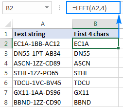
For example, to get the first 4 characters from the beginning of a text string, use this formula:
=LEFT(A2,4)
Get substring from end of string (RIGHT)
To get a substring from the right part of a text string, go with the Excel RIGHT function:
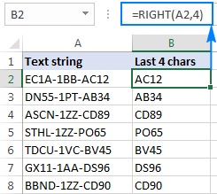
For instance, to get the last 4 characters from the end of a string, use this formula:
=RIGHT(A2,4)
Extract text from middle of string (MID)
If you are looking to extract a substring starting in the middle of a string, at the position you specify, then MID is the function you can rely on.
Compared to the other two Text functions, MID has a slightly different syntax:
Aside from text (the original text string) and num_chars (the number of characters to extract), you also indicate start_num (the starting point).
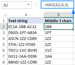
In our sample data set, to get three characters from the middle of a string beginning with the 6th character, you use the following formula:
=MID(A2,6,3)
Tip. The output of the Right, Left and Mid formulas is always text, even when you are extracting a number from a text string. If you want to operate on the result as a number, then wrap your formula in the VALUE function like this:
=VALUE(MID(A2,6,3))
Extract substring before or after a given character
As shown in the above examples, the Left, Right and Mid functions cope nicely with uniform strings. When you are dealing with text strings of variable length, more complex manipulations shall be needed.
Note. In all of the below examples, we will be using the case-insensitive SEARCH function to get the position of a character. If you want a case-sensitive formula, use the FIND function instead.
How to extract text before a specific character
To get a substring preceding a given character, two things are to be done: first, you determine the position of the character of interest, and then you pull all characters before it. More precisely, you use the SEARCH function to find the position of the character, and subtract 1 from the result, because you don't want to include the character itself in the output. And then, you send the returned number directly to the num_chars argument of the LEFT function:
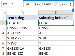
For example, to extract a substring before the hyphen character (-) from cell A2, use this formula:
=LEFT(A2, SEARCH("-",A2)-1)
No matter how many characters your Excel string contains, the formula only extracts text before the first hyphen:
How to extract text after character
To get text following a specific character, you use a slightly different approach: get the position of the character with either SEARCH or FIND, subtract that number from the total string length returned by the LEN function, and extract that many characters from the end of the string.
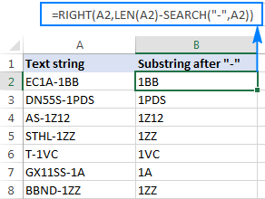
In our example, we'd use the following formula to extract a substring after the first hyphen:
=RIGHT(A2,LEN(A2)-SEARCH("-",A2))
How to extract text between two instances of a character
To get a substring between two occurrences of a certain character, use the following generic formula:
The first two arguments of this MID formula are crystal clear:
Text is the cell containing the original text string.
Start_num (starting point) - a simple SEARCH formula returns the position of the desired character, to which you add 1 because you want to start extraction with the next character.
Num_chars (number of chars to extract) is the trickiest part:
- First, you work out the position of the second occurrence of the character by nesting one Search function within another.
- After that, you subtract the position of the 1st occurrence from the position of the 2nd occurrence, and subtract 1 from the result since you don't want to include the delimiter character in the resulting substring.
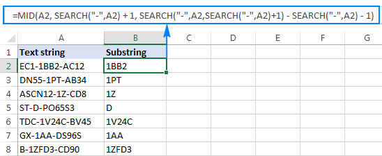
For example, to extract text surrounded by two hyphens, you'd use this formula:
=MID(A2, SEARCH("-",A2) + 1, SEARCH("-",A2,SEARCH("-",A2)+1) - SEARCH("-",A2) - 1)
The screenshot below shows the result:
If you are looking to extract text between 2nd and 3rd or 3nd and 4th occurrences of the same character, you can use a more compact SEARCH SUBSTITUTE combination to get the character's position, as explained in How to find Nth occurrence of a character in a string:
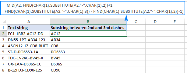
In our case, we could extract a substring between the 2nd and 3rd hyphens with the following formula:
=MID(A2, FIND(CHAR(1),SUBSTITUTE(A2,"-",CHAR(1),2))+1, FIND(CHAR(1),SUBSTITUTE(A2,"-",CHAR(1),3)) - FIND(CHAR(1),SUBSTITUTE(A2,"-",CHAR(1),2))-1)
How to find substring in Excel
In situations when you don't want to extract a substring and only want to find cells containing it, you use the SEARCH or FIND function as shown in the above examples, but perform the search within the ISNUMBER function. If a cell contains the substring, the Search function returns the position of the first character, and as long as ISNUMBER gets any number, it returns TRUE. If the substring is not found, the search results in an error, forcing ISNUMBER to return FALSE.
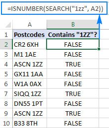
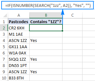
Supposing, you have a list of British postcodes in column A and you want to find those that contain the substring "1ZZ". To have it done, use this formula:
=ISNUMBER(SEARCH("1zz", A2))
The results will look something similar to this:
If you'd like to return your own message instead of the logical values of TRUE and FALSE, nest the above formula into the IF function:
=IF(ISNUMBER(SEARCH("1zz", A2)), "Yes", "")
If a cell contains the substring, the formula returns "Yes", an empty string ("") otherwise:
As you may remember, the Excel SEARCH function is case-insensitive, so you use it when the character case does not matter. To get your formula to distinguish the uppercase and lowercase characters, opt for the case-sensitive FIND function.
For more information on how to find text and numbers in Excel, please see If cell contains formula examples.
How to extract text from cell with Ultimate Suite for Excel
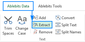
As you have just seen, Microsoft Excel provides an array of different functions to work with text strings. In case you are unsure which function is best suited for your needs, commit the job to our Ultimate Suite for Excel. With these tools in your Excel's arsenal, you just go to Ablebits Data tab > Text group, and click Extract:
Now, you select the source cells, and whatever complex strings they contain, a substring extraction boils down to these two simple actions:
- Specify how many characters you want to get from the start, end or middle of the string; or choose to extract all text before or after a given character.
- Click Insert Results. Done!
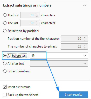
For example, to pull the domain names from the list of email addresses, you select the All after text radio button and type @ in the box next to it. To extract the user names, you select the All before text radio button, as shown in the screenshot below.
And you will get the following results in a moment:

Apart from speed and simplicity, the Extract Text tool has extra value - it will help you learn Excel formulas in general and substring functions in particular. How? By selecting the Insert as formula checkbox at the bottom of the pane, you ensure that the results are output as formulas, not values.
In this example, if you select cells B2 and C2, you will see the following formulas, respectively:
- To extract username:
=IFERROR(LEFT(A2,SEARCH("@",A2)-1),"") - To extract domain:
=IFERROR(RIGHT(A2, LEN(A2)- SEARCH("@",A2) - LEN("@") + 1),"")
How much time would it take you to figure out these formulas on your own? ;)
Since the results are formulas, the extracted substrings will update automatically as soon as any changes are made to the original strings. When new entries are added to your data set, you can copy the formulas to other cells as usual, without having to run the Extract Text tool anew.
If you are curious to try this as well as many other useful features included with Ultimate Suite for Excel, you are welcome to download evaluation version.
More formulas for substrings in Excel
In this tutorial, we have demonstrated some classic Excel formulas to extract text from string. As you understand, there can be almost infinite variations of these basic scenarios. Below you will find a few more formula examples where the Text functions come in handy.
Available downloads
Excel substring functions - practice workbook (.xlsx file)
Ultimate Suite - trial version (.exe file)
 by
by
425 comments
Hi,
I want to extract the just the website address and not the rest of the links. Can you help me with the formula?
Hello!
To extract the website address, try formula:
=LEFT(A1,SEARCH("#",SUBSTITUTE(A1,"/","#",3)))
Hello,
Are you able to extract the last bit for me, i.e. '1453510'
/CODE/ZZ/PARIS-LONDON/89853323/1453510
Many Thanks,
=RIGHT($B2,LEN($B2)-SEARCH("/",$B2,LEN($B2)-8))
Hello!
Here is the article that may be helpful to you: How to extract number from the end of text string.
I hope it’ll be helpful.
Hi,
If I want to extract just the name, what formula to use?
Farms Limited #33-1A
thanks,
Hi!
Try the following formula:
=LEFT(A1,SEARCH("#",A1)-1)
You didn't explain, but I'm guessing the name will be retrieved.
Hello Ablebits Team,
I have some data that I need to extract but can't seem to find the answer above, this is one of the cells that I need to extract a Product ID from (all cells will have varying numbers of characters) -
"adult=No,age_group=Adult,c2c_barcode=4062451243197,c2c_colour_swatch=16402,c2c_excerpt=The classic design of the Puma Road Map Golf Polo Shirt is simple enough to pair up with any golf trousers or shorts yet stylish enough to get you through your round with confidence. ,c2c_features=
dryCELL moisture-wicking technology
UPF 40 UV protection
Stretch fabric
Puma branding
80% Polyester / 15% Cotton / 5% Elastane
,c2c_mpn=595788-06,c2c_noaddtocart=0,c2c_rrp=40.00,call_for_price=No,color=Ibiza Blue/Dark Denim (PU595788-06),cross_over_id=PU59578817,default_price_of_set=0.000000,description_below_images=0,ping_popup=No,pl_size_chart=Puma Men's Clothing,price_per_unit=0,product_tag=Sale,size=S,size_system=UK,size_type=Regular"
Basically, all of the cells will include the cross_over_id= but what I need to extract is the actual cross_over_ID - in this instance it is PU59578817, is there a formula for this, please?
Hello!
The formula below will do the trick for you:
=MID(A1,SEARCH("cross_over_id=",A1)+14, SEARCH(",",A1,SEARCH("cross_over_id=",A1)+14) - (SEARCH("cross_over_id=",A1)+14))
Alexander, you are an absolute legend! Thank you.
I have a string
Maintenance Charlie 1,2590 @ 2,000 service period 4/1/2021 to 3/31/2022
I would like to extract from date in one column and end date in another column, help me how can I do that
Hello!
Divide your text into individual cells using the Extract text tool as described in the article above. You can also use the Text to Columns tool or the Split Text tool.
Hello,
I have a document coding which will be in the same format which has 3 Hyphen and 2 space and 1 dot (occasionally)
Eg for max lenght of textstring is: AAA-(BBB)-C99-DD 5555.001 (XX-YY)
Eg for min lenght of textstring is: AAA-(BB)-C8-DD 5555 (XX)
I need to print each section in the coding to a different cell. For example;
A1: AAA
A2: (BBB)
A3: C99
A4: DD
A5: 5555
A6: 001
A7: (XX-YY)
I couldn't sort it out the formula for "DD" section after last hyphen and before space and the remaining text. Thanks in advance.
Hello!
Your string is too long to be split using a formula. It also has no common pattern. Do I recommend using the Split Text tool, as described in this guide. Separate by "-" first, then by other separators. Use the Transpose tool to write the result to a column.
You can try them in trial mode.
column of data with either numbers of varying length or numbers of varying length followed by a letter. I need to split this column into 2 columns. If the cell is a number then the 1st column should simply return the number and the 2nd column will remain empty. But if the cell contains any text the 1st column will return the numbers from the cell and the second column will return any letters. Thanks so much for any help.
For instance
Col A Col B Col C
671 671
894256 894256
89G 89 G
9451w 9451 w
4589 4589
12tw 12 tw
Hello!
Use the formula from the article — How to get number from any position in a string.
To extract all letters except numbers from a cell, use the formula:
=SUBSTITUTE((CONCAT(IF(NOT(ISNUMBER(--MID(A3,ROW(INDIRECT("1:"&LEN(A3))),1))),MID(A3,ROW(INDIRECT("1:"&LEN(A3))),1),"")))," ","")
I hope my advice will help you solve your task.
1-356039-1-1-11771232_82253500
Hello,
I am trying to extract the cell right of 1-356039-1-1-, but I can't seem to get it work.
Any tips?
Hello!
If I got you right, the formula below will help you with your task:
=MID(A1,LEN("1-356039-1-1-")+1,50)
Hi ,
When I generate a report daily one coloum consist of delimited text where I need to search some keyword like (count :1) I need to get the assigned value of count .. can some one help please
Hi!
Please provide me with an example of the source data and the expected result.
Hi ,
A sample sentence has been provided below , content will be be different need to get the value of count
Eg :
This has been updated count :02 , please check
Excpeted output :02
Hello!
If I understand correctly, you need to extract the number from the text. I think this comment has an answer to your question.
I am having difficulty extracting the date listed in several items. I was only able to successfully extract the date (example 2021_02_23) when there was only one underscore proceeding it using =IF(LEN(A4)-LEN(SUBSTITUTE(A4,"_",""))=4,LEFT(RIGHT(A4,LEN(A4)-INT(FIND("_",A4)-1)-1),INT(FIND("_",RIGHT(A4,LEN(A4)-INT(FIND("_",A4))))+5)),"not in correct format")
Any feedback would be greatly appreciated.
BIO_2021_02_23_Apple
BRIEF_2021_09_28_Cat
MR_TY_2020_03_20_Apple
TAX_REC_2021_06_29_Bolton
Hello!
I recommend splitting a cell using any of the methods described in this article. Delimiter - "_". Then use the DATA function.
If you want to extract date as text use this formula:
=SUBSTITUTE(TRIM(CONCAT(IF(ISNUMBER(--MID(A1,ROW($1:$94),1)),MID(A1,ROW($1:$94),1)," ")))," ","_")
You can replace the "_" character with any other character in the formula, for example "."
Hi,
I have following texts in separate rows
TA/21-22/0001
TAS/21-22/0001
WH/TA/21-22/0001
I would like to extract the text before 0001 in each cell with a single formula. Kindly help.
Hello!
The formula below will do the trick for you:
=LEFT(A1,SEARCH("0001",A1,1)-1)
This should solve your task.
below formula in your above example is not working, tried a lot.
it should extract characters between 2nd and 3rd hypen.
output should be 3333
1111-2222-3333-4444
=MID(A2, FIND(CHAR(1),SUBSTITUTE(A2,"-",CHAR(1),2))+1, FIND(CHAR(1),SUBSTITUTE(A2,"-",CHAR(1),3)) - FIND(CHAR(1),SUBSTITUTE(A2,"-",CHAR(1),2))-1)
could you please check why the desire output not comming.
Thanks a lot
Hi!
Carefully copy the formula. Do not use — instead -
Formula works.
Hello,
I've got multiple columns each with data like so "a2b3c1"
eg A1: a2c1
B1: a3
C1: z2a4b5c1
Only one digit will ever follow a letter
What would be a formula to find and then sum the digit after "a" (eg 2+3+4=9)?
I hope this makes sense
Hello!
If I understand your task correctly, the following formula should work for you:
=SUM(--MID(A1:A4,SEARCH("a",A1:A4)+1,1))
Hi -
I am trying to extract certain words from a lookup table. For example:
Cell A1: Q1 Intelliquip invoice
Cell A2: Q2 Intelliquip
Cell A3: Intelliquip - RJE
I am trying to look at cells A1:A3 and find the word "intelliquip", based on a full list elsewhere, and just return the word "Intelliquip". I've found that i can do this for A1: =IFERROR(RIGHT($A1,LEN($A1)-SEARCH($CA$2:$CA$188,$A1)+1),0), however, this would include everything after the world Intelliquip, when i just want that word.
Thoughts on how to return just the specific word i'd like, when there is no structure in the cell i'm trying to find?
Thanks!
Logan
Hello!
I’m sorry but your description doesn’t give me a complete understanding of your task. Your formula is not working. Correct me if I’m wrong, but I believe the formula below will help:
=IF(ISNUMBER(SEARCH("Intelliquip",A1)),"Intelliquip","")
Yes, that formula would be ok. However, I'm hoping for it to be multiple lookups other than just Intelliquip (other vendors, etc.). So that is why I was hoping to do a search(look up to a list of words I want). That way, I can just drag the formula down and it will output the one-word Vendor for me. So it would capture Intelliquip below, as well as Water Systems Council (just two examples) since that lookup table will have those words in there.
Cell A1: Q1 Intelliquip invoice
Cell A2: Q2 Intelliquip
Cell A3: Intelliquip - RJE
Cell A4: Water Systems Council invoice
Cell A5: Q2 Water Systems Council
Cell A5: Water Systems Council - RJE
Hi!
You can combine these conditions in one formula if you study how to use the nested IF function in Excel to check multiple conditions.
Hope this is what you need.
Hello,
I have a plea at you I have output from database looks like this:
virtual_eth_adapters=2/0/90//0/0/SWITCH//all/none,9/0/90//0/0/SWITCH//all/none
to create a working text for further processing I need to get into this format. Basically, add two backslashes and two " to separate two parameters and add backslash \ and quotation mark " at the beginning and end of text.
\"virtual_eth_adapters=\"\"2/0/90//0/0/SWITCH//all/none\"\",\"\"9/0/90//0/0/SWITCH//all/none\"\"\",
Any idea?
Hi,
I found a solution to do it in three parts:
add characters to the end of string
change characters in the middle of string
and update the starting element.
here are my functions, however, I am not able to combine them into one big nested function
end of string: =(REPLACE(C32;LEN(C32);1;"e\""\""\"""))
middle of string: =(REPLACE(C32;FIND(",";C32);1;"\""\"",\""\"""))
beginning of string: =(REPLACE(C32;1;21;"\""virtual_fc_adapters=\""\"""))
Thank you for any help
I need to retrieve the text with two conditions
MS16-057: Security Update for Windows Server 2012 R2 (KB3156059)
condition 1 : MS16-057
condition 2 : Windows Server 2012
Need print this (KB3156059) separate cell if above condition is statisfied.
Hello!
I hope you have studied the recommendations in the tutorial above. It contains answers to your question.
Use paragraph: "How to find substring in Excel" and "How to extract text after character"
cell 1: UPENDRA C. UPRETI (6710)
cell 2: B.S.ARUNACHALAM (6503)
Dear Sir, i want to extract (only name i.e text) not the extension no.
Hello!
To extract only text without brackets from a cell, use the formula
=SUBSTITUTE(SUBSTITUTE((CONCAT(IF(NOT(ISNUMBER(--MID(A1,ROW($1:$93),1))),MID(A1,ROW($1:$93),1),"")))," ",""),"()","",1)
This should solve your task.
Hello, I have trouble finding a suitable formulas to merge a piece of text from two cells into one cell.
cell A1: RU_2017_4 DHL Automotive, IČO: 05164581
cell B1: s.r.o. (EX-04577)
the result should be: DHL Automotive, s.r.o.
Thank you!
Hello!
The formula below will do the trick for you:
=MID(A1,SEARCH(" ",A1,1)+1,SEARCH(",",A1,1)-SEARCH(" ",A1,1)+1)&LEFT(B1,6)
Hope this is what you need.
I need to exctract the string {SYS:}}{S:{MAN:CFS FILTER}{SIG:210601AMH_STP431259368}} from
{1:F01CFSMAU2SAXXX0908456442}{2:O0811400210531EAEAXXXXGXXX00363006232106010000S}{4:{202:0001}{203:0001}{305:A}{332:000000000000}}{5:{CHK:1853274C0ADA}{SYS:}}{S:{MAN:CFS FILTER}{SIG:210601AMH_STP431259368}}
would some one be able to assist?
Hi!
If I got you right, the formula below will help you with your task:
=MID(A2,SEARCH("{SYS:}",A2,1),200)
Hope this is what you need.
Hi, i have a query that i have a vehicle's data where different models are mentioned in each line of a same company and i want to extract exactly those.
1 UNIT(S) USED CAR(S) 2017 MITSU MINICAB CH/NO:
1 UNIT(S) USED VEHICLE MITSU EK WAGON CHASSIS NO :
these are data in 2 different lines and i want in next column that it should show me either Mini cab or EK Wagon
Hello!
It is possible to extract the name of the car from the text by the mask. The name of the car must be enclosed in some characters. Or there must be some pattern in the text. I don't see any of this.
This is very helpful, thank you!
What formula we can use to take a number in line after a word
Ex Biscuit 500
Biscuit 600
Biscuit 700
I want only numbers to taken in different coulum
As I mentioned numbers which is Available after common word biscuit
Hello!
The formula below will do the trick for you:
=SUMPRODUCT(MID(0&A1, LARGE(INDEX(ISNUMBER(--MID(A1, ROW(INDIRECT("1:"&LEN(A1))), 1)) * ROW(INDIRECT("1:"&LEN(A1))), 0), ROW(INDIRECT("1:"&LEN(A1))))+1, 1) * 10^ROW(INDIRECT("1:"&LEN(A1)))/10)
How can I extract "TG" from the following:
EVERGREEN: HNTB Holdings ltd - TG Only 1/1/2022
Hi!
I’m sorry but your description doesn’t give me a complete understanding of your task. Correct me if I’m wrong, but I believe the formula below will help:
=IF(ISNUMBER(SEARCH("TG",A1,1)),"TG","")
hi! I have a data written in (Name | DGL | Capacity | DISCO) i have to extract the DISCO from the cell but my All excel sheet and data is not in this format some are of other format Can you please tell the formula from which i can extract DISCOs where they are written and left the other cells blank where the discos are not written
Thank you,,,thank you,,,,thank you for your tips. By reading all pertinent examples (LEFT, RIGHT, MID and so on) on how to extract (or seek the presence of a substring in a cell ) was able to get rid of unwanted old data in my worksheet using the SEARCH function. The SEARCH function gave me a TRUE or FALSE value according to the match and then I sorted and got rid of all TRUE conditions. Kudos to You. You are the expert.
I have a state data... The template
An Anambra state
Be Benue
FC Federal capital Territory
Cr cross River state
EJ Ekiti
And I want to extract the state name only..
Anambra
Benue
Federal capital Territory
Cross River
Ekiti
How can I do this
Hello!
If I got you right, the formula below will help you with your task:
=SUBSTITUTE(MID(A1,SEARCH(" ",A1,1)+1,50),"state","")
I hope it’ll be helpful.
Dear All,
please any one can help me to post some basic excel formulas.
Thanks a lot
Hello,
I am working on simplifying my excel spreadsheet for work and I cannot seem to come up with the right function.
My spreadsheet looks like a list of employees. I need to be able to take the first letter of the first name, the fourth letter of the first name then the first letter of the last name and the fourth letter of the last name and put it into another cell.
Ex. if the name is Robert Michaelson, I need 'REMH' to be extracted from it. Does anyone know how to do this?
Thanks!
Hello,
I'm working on a proyect that requieres to extract a 4 digits code from the raw data, I found it out using the formula: =MID(E2,FIND("-",E2)+2,4) and it worked perfectly for this template:
Akbar, Bethany - w4x1 ^
Acosta, Sandra - m9ii
Slate, David - h3as
Sheppard, Jilliam - J0LW ^
The formula returns 4 digits code after "-" and " " (Space)... I got w4x1, m9ii, h3as, J0LW...
But did not returned the correct code on othis case:
Baker-Hudson, Alexis - j2mg
The reason is because this template contains 2 "-" insted of one.
What would you suggest? Is there any way I get get all of them right? I'll highly appreciate your help.
Hello!
The formula below will do the trick for you:
=MID(SUBSTITUTE(E2,"-","#", LEN(E2)-LEN(SUBSTITUTE(E2,"-",""))), FIND("#",SUBSTITUTE(E2,"-","#", LEN(E2)-LEN(SUBSTITUTE(E2,"-",""))))+2,4)
I hope my advice will help you solve your task.
I am not able to registration number from the sentence. I.e. AA01WW1111 TO ZZ11WW1111. Every time I am using mid and find formula with changing first two letters to pick registration numbers. Is there any alternate?
Hi,
I’m sorry but your task is not entirely clear to me. Could you please describe it in more detail? What result do you want to get? What formula are you using?
Hi,
I am not able to get the 10 digit registration numbers from a sentence. Its contains various state registration numbers in each cell. At present, I am using the below formula.
=mid(find,a1("AA",A1,1),10) to get AA10DE1234 from the sentence.
Hello!
If your text is AA01WW1111 TO ZZ11WW1111, then you can extract both codes using the formula
=MID(A1,FIND({"AA","ZZ"},A1,1),10)
Hope this is what you need.
Hi
Thanks for your support. I wish to bring your notice that i want to find the codes between AA01AA0000 TO ZZ99ZZ0000. In this connection I have to fetch the first two characters which contains from AA to ZZ in a cell.
I furnish below the table for your references.
TEXT IN THE SENTENCE USED FORMULA RESULT
AA01DD1234 =MID(B3,FIND("AA",B3,1),10) AA01DD1234
AB01DD1234 =MID(B4,FIND("AA",B4,1),10) #VALUE!
AC01DD1234 =MID(B5,FIND("AA",B5,1),10) #VALUE!
BC01DD1234 =MID(B6,FIND("AA",B6,1),10) #VALUE!
DC03BD3214 =MID(B7,FIND("AA",B7,1),10) #VALUE!
Hello!
If I understand your task correctly, the following formula should work for you:
=CONCAT(IFERROR(MID(A1,FIND(K1:K20,A1,1),10),""))
K1:K20 - range with the desired values - AA, ZZ, etc. There should be no empty cells.
If there is anything else I can help you with, please let me know.
Is it possible to search for either of 2 substrings? I.e. if the text contains Orange OR Blue? I'm using this as a baseline to find one substring:
=IF(ISNUMBER(SEARCH("1zz", A2)), "Yes", "")
But, I need to see if another option exists as well. Either substring would be a positive result in my case.
Hello!
If I understand your task correctly, the following formula should work for you:
=IF(OR(ISNUMBER(SEARCH("1zz", A2)),ISNUMBER(SEARCH("2zz", A2))), "Yes", "")
I hope it’ll be helpful.
How can extract "Omkarbhai" bhai in first column and second column "Omkarben" how can extract ben,
formula will apply one column. So it is possible or not. please share a logic please.
Hello!
Please check the formula below, it should work for you:
=SUBSTITUTE(A1,"Omkar","",1)
How to get selected characters from string like below
if i need to get 3rd & 5th say "RE" character from below how will i get
E9LRHE1719
Just correction
3rd & 5th are LH
Hello!
Sorry, it's not quite clear what you are trying to achieve.
Specify what you want to do. What result do you want to get? R and E is 4 and 6 characters. To extract 3 and 5 characters, you can use the MID function
=MID(E1,3,1)&MID(E1,5,1)
Hi,
I would like to extract the text AFTER the second hyphen eliminating the any space to show just the text (SS & Medicare tax) from the string below:
5200 · Payroll Taxes:5260 · SS & Medicare tax
Thanks in advance!
Hello!
Determine the position of the second hyphen using the formula
=SEARCH("· ",C1,SEARCH("· ",C1)+1)
Then use this position in MID function
=MID(C1,SEARCH("· ",C1,SEARCH("· ",C1)+1)+2,100)
Awesome, thank you!
ASCN12-1Z-CD8,BHFT
Hello All,
I need to extract "CD8", please anyone able to help me on this?
Thanks
Hello!
I believe the following formula will help you solve your task:
=MID(E1,FIND(",",E1,1)-3,3)
Hello!! Please help:
how can i make a formula that: from a text in a cell TO CHOOSE the 3rd to 5th string AND at the same time the same product NOT TO BE repeated in the column AND IF repeated then CHOOSE THE NEXT consonant (not a vowel) AND IF reapeted (given the above formula) THEN SUBSTITUDE with numbers in row 1,2,3 etc?? ?
Hello!
Unfortunately, without seeing your data it is difficult to give you any advice. Please provide me with an example of the source data and the expected result.
Halo!
I am this string of text and would like to extract out the consultation remarks and when I tried using the MID function, I am unable to get the remarks. Possible to help? Thanks
RegistrationId : NYHAE20200820, ConsultationRemark : Testing right side of LHR,CreatedBy : Scott_Reynolds, CreatedDate: 22/8/2020 12:59:31 PM,UpdatedBy : Scott_Reynolds, UpdatedDate: 22/8/2020 12:59:31 PM
Hello!
I’m sorry but your task is not entirely clear to me. Could you please describe it in more detail? What result do you want to get? Thank you!
i didn't got what i am looking
i wants to extract number from a string
i have extracted text to columns
my name is gopal sharma and i my mobile number is 0011223344)* with me
your name is unknown and 0011223345) is your contact number
number could be in any cell
how could i extract if i have different numbers
Hello!
To extract all numbers from text, use the formula
=SUMPRODUCT(MID(0&A1, LARGE(INDEX(ISNUMBER(--MID(A1, ROW(INDIRECT("1:"&LEN(A1))), 1)) * ROW(INDIRECT("1:"&LEN(A1))), 0), ROW(INDIRECT("1:"&LEN(A1))))+1, 1) * 10^ROW(INDIRECT("1:"&LEN(A1)))/10)
I hope my advice will help you solve your task.
Hi,
Thank you for your sharing. I used this formula and it's work! It's so helpful.
But there's something problem that I found in my case. That is, how if I want extract numbers from text but with the decimal ?
for example, I want extract: "ABCD 19.50PQR XTV" and "DCBA GHT KLM 99.90HV"
should be: "19.50" and "99.90"
Please help me. Thank you
Hi!
To extract a number with a decimal separator from text, try this formula:
=TEXTJOIN("",TRUE,IFERROR(MID(A2,ROW(INDIRECT("1:"&LEN(A2))),1)*1,IF(MID(A2,ROW(INDIRECT("1:"&LEN(A2))),1)=".",".","")))
You can learn more about how to extract number from text string in Excel in this article on our blog.
Extremely useful website! Thanks for sharing.
How do I extract a specific character from a word?
eg - if the word is wate%r, how do i extract "%" from it. So if there is a list of words of different length, and different placements of "%", I need one formula which will extract the "%" from it. Result should be "%" for all words.
Hello!
If I understand your task correctly, the following formula should work for you:
=IF(ISNUMBER(FIND("%",A1,1)),"%","")
Hope this is what you need.
Thank you! this worked..
Hello,
I have a column in column A that has movie names and release dates as one text string. How do separate the movie name from the long date? I've figured out how to extract when it's only the movie name and date together, but sometimes the movie synopsis follows the date in the same column. This is where it stumps me. To split the movie and the date, when it's only those two items, I have a column for each month, and have used =iferror(left(a2,find($f$1,a2)-1),"") where f1 is the heading for January, g2 for February, h3 for March and so on through December. This has successfully given me the movie name, but in the column i have for the date, I have this formula (=text, e2,"mmmm dd, yyyy"). When the synopsis follows the date, I'm left with the date followed by a paragraph of text in that column that I can't seem to get rid of.
Thank you,
Mike
Hello!
Unfortunately, without seeing your data it hard to give you advice.
Please provide me with an example of the source data and the expected result.
It’ll help me understand your request better and find a solution for you.
is there a way to upload a snippet of my worksheet so you can see it? In essence I have one column that I want to split the date from the text. The source column would be formatted like:
Source Result Result
Column A Column B Column C
Movie nameJuly 22, 2020 Extraneous text Movie name July 22, 2020
Movie nameAugust 8,2020 Movie name August 8, 2020
Movie nameSeptember 4, 2020 Alphanumeric Movie name September 4, 2020
Movie nameMay 1, 2021 Text text text text Movie name May 1, 2021
The formatting of my reply should look nothing like that. I want three columns. The first column is for example: The King's ManSeptember 18, 2020 As a collection of history's worst tyrants and criminals....
The second column, I want to output just the movie name
The third column I want to output only the date in long format. I don't want the text that follows the date in the source column kept at all. I want to strip that and toss it away.
I want to put first four alphabets in last in the same column.
For Example want to change 4296HR55U to HR55U4296.
Pls help.
Regards
Hello!
If I understand your task correctly, the following formula should work for you:
=REPLACE(D1,1,4,"")&LEFT(D1,4)
I hope this will help
Hi Anyone can help me out extract "AHU" from "LEGTAIFIYA TVS AHU-02-A-1M"
Hello!
The information presented to you is not enough to give you advice.
Need to determine if "AHU" appears in the text? Or do you need to extract text from some position?
Please describe your problem in more detail. It’ll help me understand it better and find a solution for you. Thank you.
May I know how to extract 黃惠玲 from string "Wong Wai Ling (黃惠玲)" in cell A1?
Thanks & Best Regards,
Terry
Hello Terry!
If I understand your task correctly, the following formula should work for you:
=MID(A2,FIND("(",A2,1)+1, FIND(")",A2,1) - FIND("(",A2,1)-1)
I hope this will help
I am trying to figure out what formula I would need to use to extract a value from the middle of a string. The length of the value can change so I was looking for a function that allows me to look up between 2 different characters including a character that repeats. An example: What is the area of a 60 degree circle when the bending radius is 1/8 round to the nearest tenth.
I want to extract the 1/8, what formula would I need to use
Hello Norma!
I think that according to your requirements it’s impossible to make a formula. The fact is that in the middle of the line is also the number 60. In addition, the character "/" is not a number.
LEFT(cell, SEARCH("char", cell)-1) is wrong, its ; instead of ,
Hello!
I’m sorry but your task is not entirely clear to me. Could you please describe it in more detail? Thank you!
I just have to say Thank you so much for this article!
I want to extract the contents of all cells containing a certain substring delimited by a "," or ";".
For example:
Cell A1 contains "0", Cell B1 contains "index:1", Cell C1 contains "0", Cell D1 contains "index:2"
I want to find all the cells that contain the word "index" and when found, to extract the full contents of the cell into one cell. In the above example, I am looking for a return value index:1,index:2.
How can I do that?
I'm trying to enter the date in one cell (01-Jan-2020) column A and want excel to split it into three columns B,C,D (day, month and year). could you please help me in formula
Dear can somebody help me to extract Q amount from below string,
LON AC YTO Q125 Q100 AC YMQ Q125 AC YYZ
Thanks