When working with unstructured text data in your worksheets, you often need to parse it to retrieve relevant information. This article will teach you a few simple ways to remove any number of characters from the left or right side of a text string.
How to remove characters from left in Excel
Removing first characters from a string is one of the most common tasks in Excel, and it can be accomplished with 3 different formulas.
Remove first character in Excel
To delete the first character from a string, you can use either the REPLACE function or a combination of RIGHT and LEN functions.
Here, we simply take 1 character from the first position and replace it with an empty string ("").
In this formula, we use the LEN function to calculate the total length of the string and subtract 1 character from it. The difference is served to RIGHT, so it extracts that many characters from the end of the string.
For example, to remove the first character from cell A2, the formulas go as follows:
=REPLACE(A2, 1, 1, "")
=RIGHT(A2, LEN(A2) - 1)
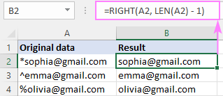
Remove characters from left
To remove leading characters from the left side of a string, you also use the REPLACE or RIGHT and LEN functions, but specify how many characters you want to delete every time:
Or
For instance, to remove first 2 characters from the string in A2, the formulas are:
=REPLACE(A2, 1, 2, "")
=RIGHT(A2, LEN(A2) - 2)
To remove first 3 characters, the formulas take this form:
=REPLACE(A2, 1, 3, "")
=RIGHT(A2, LEN(A2) - 3)
The screenshot below shows the REPLACE formula in action. With RIGHT LEN, the results would be exactly the same.

Custom function to delete first n characters
If you don't mind using VBA in your worksheets, you can create your own user-defined function to delete characters from the beginning of a string, named RemoveFirstChars. The function's code is as simple as this:
Once the code is inserted in your workbook (the detailed instructions are here), you can remove first n characters from a given cell by using this compact and intuitive formula:
For example, to delete the first character from a string in A2, the formula in B2 is:
=RemoveFirstChars(A2, 1)
To strip first two characters from A3, the formula in B3 is:
=RemoveFirstChars(A4, 2)
To delete first three characters from A4, the formula in B4 is:
=RemoveFirstChars(A4, 3)

More about Using custom functions in Excel.
How to remove characters from right
To remove characters from the right side of a string, you can also use native functions or create your own one.
Remove last character in Excel
To delete the last character in a cell, the generic formula is:
In this formula, you subtract 1 from the total string length and pass the difference to the LEFT function for it to extract that many characters from the beginning of the string.
For instance, to strip the last character from cell A2, the formula in B2 is:
=LEFT(A2, LEN(A2) - 1)
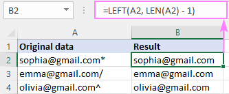
Remove characters from right
To strip off a given number of characters from the end of a cell, the generic formula is:
The logic is the same as in the above formula, and below are a couple of examples.
To remove the last 3 characters, use 3 for num_chars:
=LEFT(A2, LEN(A2) - 3)
To delete the last 5 characters, supply 5 for num_chars:
=LEFT(A2, LEN(A2) - 5)

Custom function to remove last n characters in Excel
If you'd like to have your own function for removing any number of characters from right, add this VBA code to your workbook:
The function is named RemoveLastChars and its syntax hardly needs any explanation:
To give it a field test, let's get rid of the last character in A2:
=RemoveLastChars(A2, 1)
Additionally, we'll remove the last 2 characters from the right side of the string in A3:
=RemoveLastChars(A3, 2)
To delete the last 3 characters from cell A4, the formula is:
=RemoveLastChars(A4, 3)
As you can see in the below screenshot, our custom function works brilliantly!

How to remove characters from right and left at once
In situation when you need to wipe out characters on both sides of a string, you can either run both of the above formulas sequentially or optimize the job with the help of the MID function.
Where:
- chars_left - the number of characters to delete from left.
- chars_right - the number of characters to delete from right.
Suppose you want to extract the username from a string like mailto:Sophia@gmail.com. For this, part of text needs to be removed from the beginning (mailto: - 7 characters) and from the end (@gmail.com - 11 characters).
Serve the above numbers to the formula:
=MID(A2, 7+1, LEN(A2) - (7+10))
…and the result won't keep you waiting:
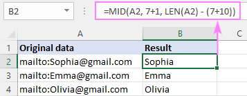
To understand what's actually going on here, let's recall the syntax of the MID function, which is used to pull a substring of a certain size from the middle of the original string:
The text argument does not raise any questions - it's the source string (A2 in our case).
To get the position of the first character to extract (start_num), you add 1 to the number of chars to be stripped off from left (7+1).
To determine how many characters to return (num_chars), you calculate the total of removed characters (7 + 11) and subtract the sum from the length of the entire string: LEN(A2) - (7+10)).
Get the result as number
Whichever of the above formulas you use, the output is always text, even when the returned value contains only numbers. To return the result as a number, either wrap the core formula in the VALUE function or perform some math operation that does not affect the result, e.g. multiply by 1 or add 0. This technique is especially useful when you want to calculate the results further.
Suppose you've removed the first character from cells A2:A6 and want to sum the resulting values. Astonishingly, a trivial SUM formula returns zero. Why's that? Obviously, because you are adding up strings, not numbers. Perform one of the below operations, and the issue is fixed!
=VALUE(REPLACE(A2, 1, 1, ""))
=RIGHT(A2, LEN(A2) - 1) * 1
=RemoveFirstChars(A2, 1) + 0
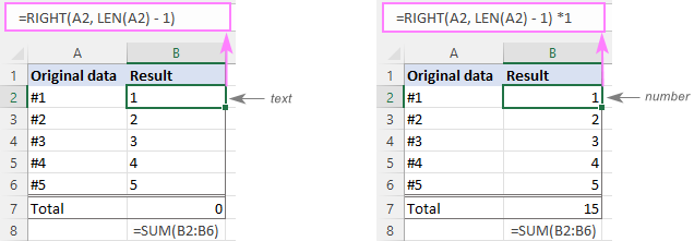
Remove first or last character with Flash Fill
In Excel 2013 and later versions, there is one more easy way to delete the first and last characters in Excel - the Flash Fill feature.
- In a cell adjacent to the first cell with the original data, type the desired result omitting the first or last character from the original string, and press Enter.
- Start typing the expected value in the next cell. If Excel senses the pattern in the data you are entering, it will follow the same pattern in the rest of the cells and display a preview of your data without the first / last character.
- Just hit the Enter key to accept the preview.

Remove characters by position with Ultimate Suite
Traditionally, the users of our Ultimate Suite can handle the task with a few clicks without having to remember a handful of various formulas.
To delete the first or last n characters from a string, this is what you need to do:
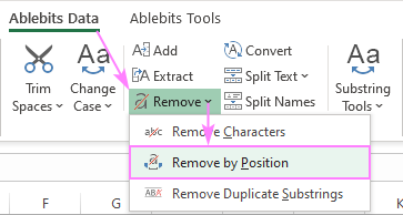
- On the Ablebits Data tab, in the Text group, click Remove > Remove by Position.
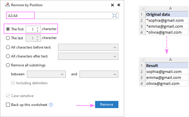
- On the add-in's pane, select the target range, specify how many characters to delete, and hit Remove.
For example, to remove the first character, we configure the following option:
That's how to remove a substring from left or right in Excel. I thank you for reading and look forward to seeing you on our blog next week!
Available downloads
Remove first or last characters - examples (.xlsm file)
Ultimate Suite - trial version (.exe file)
 by
by
34 comments
This solved my problem exactly! Thank you!
Thank you so much for the detailed explanations and examples. Made a small registry Key - value divider thanks to your mid function example.
So helpful!
ERS-24N017S0291JH003-2331985 -- This is my string and I want to pick up "24N017S0291JH003"
Hi! For your problem, we can offer several solutions. Look for the example formulas here: Get text between two instances of the same character in Excel.
=MID(A2, SEARCH("-", A2) +1, SEARCH("-", A2, SEARCH("-",A2) +1) - SEARCH("-", A2) -1)
With the TEXTSPLIT function, you can split text into individual cells. For example, by using the "-" separator.
=TEXTSPLIT(A2,"-")
You can use the CHOOSECOLS function to select a second word:
=CHOOSECOLS(TEXTSPLIT(A2,"-"),2)
Our Extract text tool may help you solve it in a few clicks. It allows you to extract substrings, text characters and digits from one Excel cell to another without formulas. It is available as a part of our Ultimate Suite for Excel that you can install in a trial mode and check how it works for free.
If I want to remove the initials (single alphabet) from a name, how can it be done.
Name Example:
L Roy
M David
K Lynus
Desired Result:
Roy
David
Lynus
Hi! Try to follow the recommendations from these guides: How to extract last word in Excel or Split first and last names into separate columns.
For example:
=RIGHT(A1,LEN(A1)-SEARCH(" ",A1,1))
Hi!
I have a list of couple thousands of products, where I need to pick up/separate the last digits from the cell. There is always the same separator „-„, however it shows up different number of times in the cell.
Example:
AA04052-11 (need 11)
IP-jd1010-20 (need 20)
Nnwd-io-20201020-9 (need 9)
1030-5 (need 5)
192028-thru-2019-5 (need 5)
I’ve tried using left/right functions combined with LEN, Search and text to columns, but still doing something wrong and getting wrong results…
I’ll be more than grateful for your help!
Thanks,
John
Hi! To extract the text after the last '-' delimiter, use these instructions: Get last word from string. Based on your information, the formula might look something like this:
=TRIM(RIGHT(SUBSTITUTE(A1, "-", REPT(" ", LEN(A1))), LEN(A1)))
Great thanks!
I have a cloumn with names as follows Last name first name and inital for some names,
I want to remove from the ones with an initial the initial and the space befor it. How can i get it done,
PS not evrey one has an inital.
Hi! To ensure clear understanding of your task, can you provide an example of the source data and the desired result you are aiming for?
You mean like:
Matthew L
Samuel
Frank K
Fred
Hello! Use the SEARCH function to get the position of the space, and the LEFT function to extract the characters up to the first space. Or you can extract a text string from text in a couple of clicks without formulas using 8 tools to manage text data in Excel. It is available as a part of our Ultimate Suite for Excel that you can install in a trial mode and check how it works for free.
=IFERROR(LEFT(A1,SEARCH(" ",A1)-1),A1)
Hi,
I have an imported set of numerical data (in columns) taken from an email (which said it was formatted for copy and paste to excel) - I copied and pasted it to a new spreadsheet - some of it pastes as text and some as numbers. I've tried various methods to convert the text to numbers from the simple format commands to copying and pasting as a value.
I tried the various methods suggested above to remove the 9 additional spaces that appear next to the numbers in each cell (that is formatted as text). Also not working.
Each time I try a new solution, when identifying the cell using =isvalue(cell) it returns a #NAME? as the answer.
Please help.
Hi! Try to change string to number with mathematic operations. I'd recommend you to have a look at our Convert Text tool that can help you convert numbers stored as text to numbers. It is available as a part of our Ultimate Suite for Excel that you can install in a trial mode and check how it works for free.
successful!
Thank you this was very helpful and saved me alot of time.
Hi,
How do i delete all the numbers which ends after the characters.
X_UcHdfadf_cusPflRjhfjgsTknNr_1266255728672168989_0
X_adfmcHm_emdghlAdTe_array_LOWER_12323144750471599279_0
X_adfmcHm_etyphnNr_array_1662712933577636652_0
X_UdfHm_dghcTknsRgsNr_enlStsCd_recStsTypCd_3394788709178767897_0
Hi!
If I understand your task correctly, the following formula should work for you:
=LEFT(A2,SEARCH("#",SUBSTITUTE(A2,"_","#",LEN(A2)-LEN(SUBSTITUTE(A2,"_",""))-1)))
Try to follow the recommendations from this article: Excel substring: how to extract text from cell.
Very helpful, appreciate the time taken to write this.
I am trying solve is text in a cell ends with "--" or "-" then make it ""
1-2-3-- becomes 1-2-3
1-2-3- becomes 1-2-3
I can fix "--" with substitute, but when I try "-" then it becomes 123, i only want to clean the end characters.
Hello i succeeded with the formula but now i want to remove the old column and keep only the new one but everytime i do it removes the values of the new one too like theyre linked?
Hi!
Look closely at your formulas and references.
Hello
I linked a cell "SHEET1'! A2" on sheet 2.
Could I link another cell (ex: "SHEET1'! A32") on sheet 2 using above linked cell reference by formula.
Thanks
Hi i am trying to delete the time in all my cells and keep only the date (22/06/2015 18:13:00) as it is disrupting my pivot table, how could i delete the time in all the cells?
Hello!
Since the date and time in Excel are numbers, round up to an integer to remove the time from the date. Use the INT rounding function.
how do i tell excell to remove all digits from the left when the number is more than 11 digits? for example N456789002234, it would remove the N4. Also, to add preceeding zeros to make the number 11 digits.
I need it to do this to a column in my excell sheet
Thank you
Hello!
To extract the 11 characters from the right, use the RIGHT function.
To make the number 11 digits, use this guide: How to add leading zeros in Excel.
Try this formula:
=TEXT(RIGHT(A1,11),"00000000000")
I hope I answered your question. If something is still unclear, please feel free to ask.
Please can any1 help me
i have 2 different number formatting 1.970.00 and € 1,970.00
how can i replace 1.970.00 first (1.9) point to coma ( , ) ?
advanced thanks
Hello!
If your number 1.970.00 is written as text, use the SUBSTITUTE function to replace the dot with a comma.
=SUBSTITUTE(A1,".",",",1)
To change the number format, use this guide: Custom Excel number format and Excel format for number, text, scientific notation, accounting.
Thank you!
Thank you for the tutorial, it really helped me a lot.
Formula work with ; and not with , in Office 365
Hi Hrvoje,
That depends on the List separator set in your Windows Regional settings. In the USA, UK and some other English-speaking countries, it's a comma. In most European countries, the default list separator is a semicolon because a comma is used as the decimal point.