The tutorial shows how to use VLOOKUP formula in Excel to compare two columns to return common values (matches) or find missing data (differences).
When you have data in two different lists, you may often need to compare them to see what information is missing in one of the lists or what data is present in both. Comparison can be done in many different ways - which method to use depends on exactly what you want from it.
How to compare two columns in Excel using VLOOKUP
When you have two columns of data and want to find out which data points from one list exist in the other list, you can use the VLOOKUP function to compare the lists for common values.
To build a VLOOKUP formula in its basic form, this is what you need to do:
- For lookup_value (1st argument), use the topmost cell from List 1.
- For table_array (2nd argument), supply the entire List 2.
- For col_index_num (3rd argument), use 1 as there is just one column in the array.
- For range_lookup (4th argument), set FALSE - exact match.
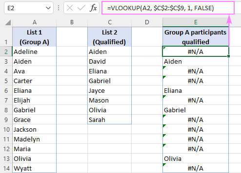
Suppose you have the names of participants in column A (List 1) and the names of those who have passed through the qualification rounds in column B (List 2). You want to compare these 2 lists to determine which participants from Group A made their way to the main event. To do this, use the following formula.
=VLOOKUP(A2, $C$2:$C$9, 1, FALSE)
The formula goes to cell E2, and then you drag it down through as many cells as there are items in List 1.
Please notice that table_array is locked with absolute references ($C$2:$C$9) so that it remains constant when you copy the formula to the below cells.
As you can see, the names of the qualified athletes show up in column E. For the remaining participants, a #N/A error appears indicating that their names are not available in List 2.
Disguise #N/A errors
The VLOOKUP formula discussed above perfectly fulfills its main objective - returns common values and identifies missing data points. However, it delivers a bunch of #N/A errors, which may confuse inexperienced users making them think that something is wrong with the formula.
To replace errors with blank cells, use VLOOKUP in combination with the IFNA or IFERROR function in this way:
=IFNA(VLOOKUP(A2, $C$2:$C$9, 1, FALSE), "")
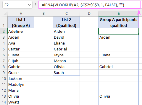
Our improved formula returns an empty string ("") instead of #N/A. You can also return your custom text such as "Not in List 2", "Not present", or "Not available". For example:
=IFNA(VLOOKUP(A2, $C$2:$C$9, 1, FALSE), "Not in List 2")
That is the basic VLOOKUP formula to compare two columns in Excel. Depending on your particular task, it can be modified as shown in further examples.
Compare two columns in different Excel sheets using VLOOKUP
In real life, the columns you need to compare are not always on the same sheet. In a small dataset, you can try spotting the differences manually by viewing two sheets side by side.
To search in another worksheet or workbook with formulas, you have to use external reference. The best practice is to start typing the formula in your main sheet, then switch to the other worksheet and select the list using the mouse - an appropriate range reference will be added to the formula automatically.
Assuming List 1 is in column A on Sheet1 and list 2 is in column A on Sheet2, you can compare two columns and find matches using this formula:
=IFNA(VLOOKUP(A2, Sheet2!$A$2:$A$9, 1, FALSE), "")

For more information, please see:
Compare two columns and return common values (matches)
In the previous examples, we discussed a VLOOKUP formula in its simplest form:
=IFNA(VLOOKUP(A2, $C$2:$C$9, 1, FALSE), "")
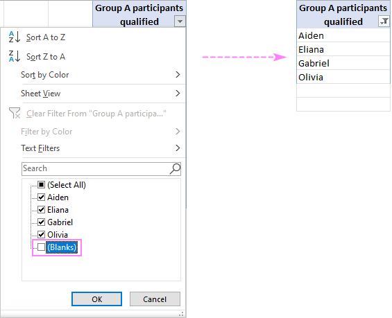
The result of that formula is a list of values that exist in both columns and blank cells in place of the values not available in the second column.
To get a list of common values without gaps, just add auto-filter to the resulting column and filter out blanks.
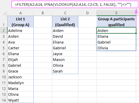
In Excel for Microsoft 365 and Excel 2021 that support dynamic arrays, you can make use of the FILTER function to sift out blanks dynamically. For this, utilize the IFNA VLOOKUP formula as the criteria for FILTER:
=FILTER(A2:A14, IFNA(VLOOKUP(A2:A14, C2:C9, 1, FALSE), "")<>"")
Please pay attention that in this case we supply the entire List 1 (A2:A14) to the lookup_value argument of VLOOKUP. The function compares each of the lookup values against List 2 (C2:C9) and returns an array of matches and #N/A errors representing missing values. The IFNA function replaces errors with empty strings and serves the results to the FILTER function, which filters out blanks (<>"") and outputs an array of matches as the final result.
Alternatively, you can use the ISNA function to check the result of VLOOKUP and filter the items evaluating to FALSE, i.e. values other than #N/A errors:
=FILTER(A2:A14, ISNA(VLOOKUP(A2:A14, C2:C9, 1, FALSE))=FALSE)
The same result can be achieved with the XLOOKUP function, which makes the formula even simpler. Due to the ability of XLOOKUP to handle #N/A errors internally (optional if_not_found argument), we can do without the IFNA or ISNA wrapper:
=FILTER(A2:A14, XLOOKUP(A2:A14, C2:C9, C2:C9,"")<>"")
Compare two columns and find missing values (differences)
To compare 2 columns in Excel to find differences, you can proceed in this way:
- Write the core formula to search for the first value from List 1 (A2) in List 2 ($C$2:$C$9):
VLOOKUP(A2, $C$2:$C$9, 1, FALSE)
- Nest the above formula in the ISNA function to check the VLOOKUP's output for #N/A errors. In case of an error, ISNA yields TRUE, otherwise FALSE:
ISNA(VLOOKUP(A2, $C$2:$C$9, 1, FALSE))
- Use the ISNA VLOOKUP formula for the logical test of the IF function. If the test evaluates to TRUE (#N/A error), return a value from List 1 in the same row. If the test evaluates to FALSE (a match in List 2 is found), return an empty string.
The complete formula takes this form:
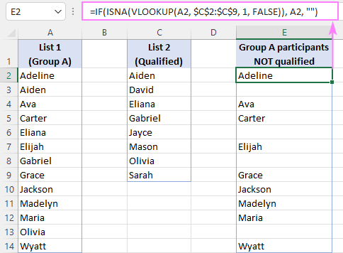
=IF(ISNA(VLOOKUP(A2, $C$2:$C$9, 1, FALSE)), A2, "")
To get rid of the blanks, apply Excel's Filter as demonstrated in the above example.
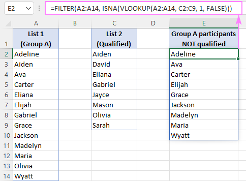
In Excel 365 and Excel 2021, you can have the result list filtered dynamically. For this, simply place the ISNA VLOOKUP formula in the include argument of the FILTER function:
=FILTER(A2:A14, ISNA(VLOOKUP(A2:A14, C2:C9, 1, FALSE)))
Another way is to use XLOOKUP for criteria - the function returns empty strings ("") for missing data points, and you filter the values in List 1 for which XLOOKUP returned empty strings (=""):
=FILTER(A2:A14, XLOOKUP(A2:A14, C2:C9, C2:C9,"")="")
VLOOKUP formula to identify matches and differences between two columns
If you want to add text labels to the first list indicating which values are available in the second list and which are not, use the VLOOKUP formula together with the IF and ISNA/ISERROR functions.
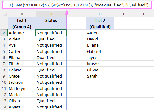
For example, to identify names that are in both columns A and D and those that are only in column A, the formula is:
=IF(ISNA(VLOOKUP(A2, $D$2:$D$9, 1, FALSE)), "Not qualified", "Qualified")
Here, the ISNA function catches the #N/A errors generated by VLOOKUP and passes that intermediate result to the IF function for it to return the specified text for errors and another text for successful lookups.
In this example, we used "Not qualified"/"Qualified" labels, which are suitable for our sample dataset. You can replace them with "Not in List 2"/"In List 2", "Not available"/"Available" or any other labels you see fit.
This formula is best to be inserted in a column adjacent to List 1 and copied through as many cells as there are items in your list.
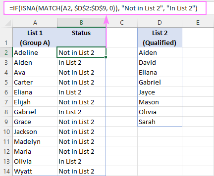
One more way to identify matches and differences in 2 columns is using the MATCH function:
=IF(ISNA(MATCH(A2, $D$2:$D$9, 0)), "Not in List 2", "In List 2")
A few other ways to accomplish the task are described in this tutorial: Check if value exists in a range.
Compare 2 columns and return a value from third
When working with tables containing related data, you may sometimes need to compare two columns in two different tables and return a matching value from another column. In fact, it is the primary use of the VLOOKUP function, the purpose it was designed for.
For example, to compare the names in columns A and D in the two tables below and return a time from column E, the formula is:
=VLOOKUP(A3, $D$3:$E$10, 2, FALSE)
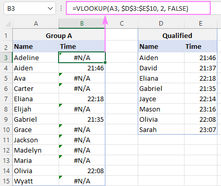
To hide #N/A errors, use the proven solution - the IFNA function:
=IFNA(VLOOKUP(A3, $D$3:$E$10, 2, FALSE), "")
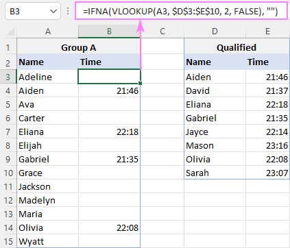
Instead of blanks, you can return any text you want for missing data points - just type it in the last argument. For instance:
=IFNA(VLOOKUP(A3, $D$3:$E$10, 2, FALSE), "Not available")
Besides VLOOKUP, the task can be fulfilled with a few other lookup functions.
Personally, I'd rely on a more flexible INDEX MATCH formula:
=IFNA(INDEX($E$3:$E$10, MATCH(A3, $D$3:$D$10, 0)), "")
Or use the modern successor of VLOOKUP - the XLOOKUP function, available in Excel 365 and Excel 2021:
=XLOOKUP(A3, $D$3:$D$10, $E$3:$E$10, "")
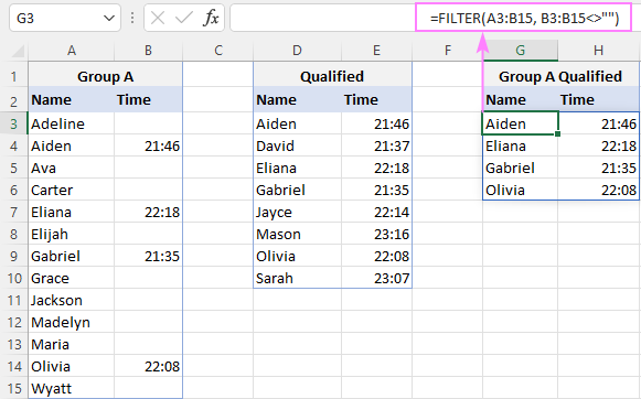
To get the names of qualified participants from group A and their results, simply filter out blank cells in column B:
=FILTER(A3:B15, B3:B15<>"")
Comparison tools
If you frequently do file or data comparison in Excel, these smart tools included in our Ultimate Suite can save your time immensely!
Compare Tables - quick way to find duplicates (matches) and unique values (differences) in any two data sets such as columns, list or tables.
Compare Two Sheets - find and highlight differences between two worksheets.
Compare Multiple Sheets - find and highlight differences in multiple sheets at once.
Practice workbook for download
VLOOKUP in Excel to compare columns - examples (.xlsx file)
 by
by
50 comments
yes confirmed I understand thanks svetlana
Hi,
I have two Excel sheets (Sheet 1 and Sheet 2) with two columns for first and last name. The data in Sheet 2 shows the same information as Sheet 1, however two people are missing. I compared them by the last name, however it brought three missing results since one of the people in Sheet 2 has changed only their last name.
How can I bring only the two missing people?
Hi! If I understand your task correctly, the following tutorial should help: Compare multiple columns for matches in the same row.
You can compare two tables without using formulas using Compare Two Tables tool. It is available as a part of our Ultimate Suite for Excel that you can install in a trial mode and check how it works for free.
how to compare 2 columns having common values one with each row of every cell
Try using the information in the article above, as well as these instructions: Compare two columns for matches and differences.
I am using this formula to find mismatches, with a checkmark for exact matches:
=IF(ISNA(VLOOKUP(D3,F3:F3340,1,FALSE)),D3,"√")
If an exact match is found, the formula returns multiple/repeating √√√√ until it completely fills the data cell.
How can I get this formula return only one checkmark (√)?
Thanks,
Sonny
Unfortunately, I could not reproduce your problem. The formula returns one character (√) if a match is found.
Maybe the problem is in the format of the cell. Read more: Repeat characters with custom format codes. Try setting the cell format to General.
first step:
Just Concatenate two column values with | separation. (ex: =Concatenate (column1 value, " | ",column2 value))
Second step:
do normal lookup formula
Hello,
i have two columns i want to compare the encounter with the clients to see if they are the same encounter # from one sheet to another sheet and see if the encounters are the same. how can i write the formula for this?
thank you in advance!
Hi!
To compare the two columns, use the guidelines in the article above. This tutorial may also be helpful: How to compare two columns in Excel for matches and differences.
Hi there,
I need some help on how to calculate hours for a client. There are two clients here, each with more than one CancelDescriptions. How can I add hours altogether for each client with data from multiple columns with Cells like this for example
A B C D E F
Client Duration CancelDescription
Sam 7 Public Holiday
Sam 4 Staff Leave
Sam 5.5 Blanks
Sam 3 Family unavailable
Paul 4.5 Staff Leave
Paul 2.5 Blanks
Also what formula to use if new client is added to the Sheet
Hi!
If I understand the problem correctly, you can calculate the amount of hours for each customer using the SUMIFS function.
=SUMIFS(B2:B9, A2:A9, "Sam")
=SUMIFS(C2:C9, A2:A9, A2)
I hope it’ll be helpful. If something is still unclear, please feel free to ask.
Hi
I have two sheets in a workbook and I want to bring in values from the a third column.
Say I have for the month of January for Lanre figure is 750 and for same Lanre figure is 800
How do I bring this in using a lookup or any other formula?
Thanks
Lanre
Hi! I'm sorry but your description doesn't give me a complete understanding of your task. You can use the formula VLOOKUP to find the value in the second column from the value in the first column. if you need more specific advice, explain the problem in more detail.
Apologies for being vague.
Maybe this will put in it a bit more context
Sheet1 Sheet 2
Name Date Name Date Rate
Lanre o 01/11/2022 Lanre o 01/11/2022 800
Paul Mate 01/11/2022 Paul Mate 01/11/2022 750
Paul Mate 01/11/2022 545
The challenge I have is that when I use the Vlookup for example for Paul Mate who has two different Rates for November for two different projects, it's only bringing in the first rate (750) for both. Same applies to everyone who's name shows up more than once.
Apologies for being vague.
Maybe this will put in it a bit more context
Sheet1
Name Date
Lanre o 01/11/2022
Paul Mate 01/11/2022
Sheet 2
Name Date Rate
Lanre o 01/11/2022 800
Paul Mate 01/11/2022 750
Paul Mate 01/11/2022 545
The challenge I have is that when I use the VLOOKUP for example for Paul Mate who has two different Rates for November for two different projects, it's only bringing in the first rate (750) for both. Same applies to everyone who's name shows up more than once
Hello!
If you want to get all the values for the criterion you specify, I recommend using this guide: Vlookup multiple matches in Excel with one or more criteria. Hope this is what you need.
Hi Alexander
Sorry for the late reply. Many thanks for your help. This was very very useful.
Hello,
First off, thanks very much for this. It's very helpful. That being said, I'm still stumped. Here is my scenario:
I have this:
ID Name AWWN HWWN D_Name Path
5 PRACDBVV.102 60002AC0000000000000038F0002140B 60002AC000000000000003910002140B dm-94 mpathbv
4 PRACDBVV.103 60002AC000000000000003900002140B
3 PRACDBVV.104 60002AC000000000000003910002140B 60002AC000000000000003900002140B dm-95 mpathbw
6 PRACDBVV.105 60002AC000000000000003920002140B 60002AC0000000000000038F0002140B dm-96 mpathbx
I want to get to this, where AWWN and HWWN columns are matched and the data in the D_Name and Path columns sort with HWWN:
5 PRACDBVV.102 60002AC0000000000000038F0002140B 60002AC0000000000000038F0002140B dm-96 mpathbx
4 PRACDBVV.103 60002AC000000000000003900002140B 60002AC000000000000003900002140B dm-95 mpathbw
3 PRACDBVV.104 60002AC000000000000003910002140B 60002AC000000000000003910002140B dm-94 mpathbv
6 PRACDBVV.105 60002AC000000000000003920002140B
Hello!
The task can be solved using the Merge Tables tool. Copy the HWWN column to a new sheet and add data to this table where HWWN equals AWWN. For more information, please visit: How to use Merge Two Tables for Excel.
It is available as a part of our Ultimate Suite for Excel that you can install in a trial mode and check how it works for free.
Thanks very much for the prompt reply! I will give it a try.
Hello
Please share how best to share my file with you so that I can determine where I am going wrong in using VLOOKUP between two Excel Worksheet for exact match.
Kind regards,
Wilma Porter
As of Friday afternoon, Jan 13, 2023, no assistance needed at this time. I have resolved what turned out to be a formatting issue with the reference Table. Thank you.
Hi Team, the formula helps me a lot, request your guide for one additional support in Vlookup. For eg. If we have to Look up data but it does not have a value like below, the value should arrive as Blank, not zero.
Lookup Details
2180312505000 200 2180312505000 200
2180312103000 0 2180312103000
2180312351000 100 2180312351000 100
I have some data, A column is a persons name and the same name can appear multiple times, B column is a year and then C column is data that relates to that year. How can i use VLOOKUP to squish up column a without losing the data from column B&C?
Hello!
Here is the article that may be helpful to you: Vlookup multiple matches in Excel with one or more criteria. If you want to merge results in one cell, use the TEXTJOIN function.
I hope it’ll be helpful.
Hello,Sir I am not a professionalist, it is only my hobby and curiosity. If you think it is ok send the solution. Thank you
SHEET1
A B C D E F G H I J K L M N O P Q R S T
1 494 494 494 494 494 494 494 494 494 494 494 494 494
2 AB
3
4 P+T
5 21-1-2021
6 22-1-2021 P
7 23-1-2021 OT
SHEET2
A B C D E F G H I J K L M N O P
1
2 494
3 AB
4
5 21-01-2021
6 22-01-2021
7
How to get return cell value “P+T” in Sheet2 which one is in Sheet1 cell P5, criteria is matching G2 and G3 in the ROW E1,E2,..........
“VLOOKUP(E7,SHEET1!E:Z,MATCH(G2,sheet1!E1:Z1,0),MATCH(G3,sheet1!E2:Z2,0)OR using index or any other method
Thanking You
Hi!
Sorry, it's not quite clear what you are trying to achieve.
hi
please advise... i have a chart of pipe weight / meter as per their size (dia) and schedule number categories. it can be found on google easily. in first column (category1) it has pipes with dia 1", 2" and in first row (category2) it has schedule data e.g. sch10, sch.40 and in the middle area it has the corresponding values of weight e.g. for pipe dia 1" sch10 w/m is 2.09, for pipe dia 1" sch40 w/m is 2.5, for pipe dia 2" sch10 w/m is 3.93, for pipe dia 2" sch40 w/m is 5.44.
i want to make a sheet where i just select the pipe size and it's schedule and the weight / meter (w/m) shows accordingly.
Regards
Waseem Akram
Hello!
Try to use the examples and recommendations described in this article: Excel INDEX MATCH with multiple criteria. This should solve your task.
Hi,
I want to uniquely identify the row with two columns.
Suppose A2 has value 123
A3 has also 123
And B2 is X2
B3 is X3.
How can we use this in the first argument to compare
VLOOKUP(A2, $D$3:$H$10, 5, FALSE)
5th is the column I want to compare.
It has value 1,2,
IF we apply this formula, I am getting 1 in both result cell. But I want to get 1 and second row cell as 2.
Please suggest.
Regards,
Panna
Hi!
Your VLOOKUP formula is looking for the value 123 in column D. I don't know your data in the search range so I can't understand your problem and what you want to compare. Explain in more detail.
If i wanted to highlight similar text Eg; Column 1 has Luis and column 2 has Luis B and i want to highlight them both because there similar? How would i go about this?
Hello!
You can use conditional formatting to change a color of similar cells with the formula:
=ISNUMBER(SEARCH(A1,B1))+ISNUMBER(SEARCH(B1,A1))
The SEARCH function searches within text. ISNUMBER returns TRUE if the lookup was successful.
I hope my advice will help you solve your task.
Not quite working. Allow me to rephrase to avoid confusion.
I have 2 columns that run at least a hundred rows.
First column has text names on it, (EG; Luis)
Second column also has text names, (Eg; Luis B) but are not identical and need to be parsed out so I can highlight each text name on each column that has similarities?
Hi!
This formula will help you determine if a similar value exists in column B.
=SUM(--ISNUMBER(SEARCH(A1,B1:B10)))
Fuzzy Duplicates Finder can also help you determine fuzzy matches. It is available as a part of our Ultimate Suite for Excel that you can install in a trial mode and check how it works for free.
Hii
In sheet 1, column C (Owner Names) and Column D (Tenant names) are provided along with "Comments" in Column E for a city. And in sheet 2, owner names are provided in column F, and tenant names are in Column H, but comments are not provided.
Now I want, if in sheet1, any of the rows, the Owner name and tenant name exactly match with the owner's name and tenant name in Sheet2 . then the comments should be copied from sheet 1 to sheet 2 in column O. In other words, if Column C & Column D (Sheet1) = Column F & Column H (Sheet 2), then from sheet 1 column E (Comments) should be pasted in Column O in the sheet 2.
Hope I mentioned my problem correctly, please help me to generate the formula for this.
Hello!
You can find the examples and detailed instructions here: Excel INDEX MATCH with multiple criteria. You will be able to extract a value based on two criteria.
=FILTER(A1:A63, ISNA(VLOOKUP(A1:A63, C1:C32, 1, FALSE))) doesn't work. Give a solution that works, dont just post for the sake of posting
A A #SPILL!
B F #SPILL!
C G #SPILL!
D H #SPILL!
E I #SPILL!
Hi!
Your VLOOKUP formula returns an array of values. Therefore, a SPILL! error may occur. Read more about this error here: #SPILL! error in Excel - what it means and how to fix.
I don't know what you are trying to achieve with this formula. Therefore, I can not give any advice on how to fix it.
Trying to look for unique values in 2 columns. I have used trim, conditional formatting (unique values) and I am still getting highlighted text even though I can see the same number in the next column!
Hello!
I don't see your data. But I assume that your numbers differ by decimal places. If you get numbers using a formula, use round numbers.
Nice!! this worked for me for-
Excellent work guys, keep the good things coming and you would get good blessings in return from individuals like me.
=IFNA(VLOOKUP(A3, $D$3:$E$10, 2, FALSE), "") :) :)
Thanks,
Vinay S.
I like to do something like this, I have a table of about 20k items and they are being compared to a new list of items, what i like to do is
if A1 = I1
then copy comment in K1 into G1
the biggest things is that i have some items that are like 8 or 9 all of the same items. I want to ensure they match or skip to the next as it goes through them all.
How is this done without a macro
Hi!
Have you tried the ways described in this blog post? If they don’t work for you, then please describe your task in more detail, I’ll try to suggest a solution.
Here is the one more article that may be helpful to you: How to compare two columns in Excel for matches and differences.
Hi
VLOOKUP function I want both whatever in column B & column C and at the same time if any column is empty in column B & column C, need only one cell value. Hope you get my point, waiting for the solution
A B C
ID Class 1 Class 2
1 Q P
2 L
3 R
4 T
5 Y
Hi!
Sorry, I do not fully understand the task. Describe in detail what result you want to get.
Hi
In column A there are IDs of some students and in column B & column C these are name of the subjects, vlookup function if I want any ID of a student I need subjects of both if they are in both column B & C. At the same time if any subject is missing in any column these B & C then I need only one subject in vlookup function, hope you get the task. Thanks in advance
Regards
Sazedul Munna
Hi!
The information you provided is not enough to understand your case and give you any formula. However, keep in mind that the VLOOKUP function can only return values from one column. To get multiple values using VLOOKUP, use this instruction. You can use two VLOOKUP formulas to get values from two columns.
To get data from multiple columns using a formula, you can use the FILTER function.
Hi
Please advise how can I share my file with you so that I can get my expected result, thanks
Regards
Sazedul Munna