The tutorial shows how to create multiple IF statements in Excel with AND as well as OR logic. Also, you will learn how to use IF together with other Excel functions.
In the first part of our Excel IF tutorial, we looked at how to construct a simple IF statement with one condition for text, numbers, dates, blanks and non-blanks. For powerful data analysis, however, you may often need to evaluate multiple conditions at a time. The below formula examples will show you the most effective ways to do this.
How to use IF function with multiple conditions
In essence, there are two types of the IF formula with multiple criteria based on the AND / OR logic. Consequently, in the logical test of your IF formula, you should use one of these functions:
- AND function - returns TRUE if all the conditions are met; FALSE otherwise.
- OR function - returns TRUE if any single condition is met; FALSE otherwise.
To better illustrate the point, let's investigate some real-life formulas examples.
Excel IF statement with multiple conditions (AND logic)
The generic formula of Excel IF with two or more conditions is this:
Translated into a human language, the formula says: If condition 1 is true AND condition 2 is true, return value_if_true; else return value_if_false.
Suppose you have a table listing the scores of two tests in columns B and C. To pass the final exam, a student must have both scores greater than 50.
For the logical test, you use the following AND statement: AND(B2>50, C2>50)
If both conditions are true, the formula will return "Pass"; if any condition is false - "Fail".
=IF(AND(B2>50, B2>50), "Pass", "Fail")
Easy, isn't it? The screenshot below proves that our Excel IF /AND formula works right:

In a similar manner, you can use the Excel IF function with multiple text conditions.
For instance, to output "Good" if both B2 and C2 are greater than 50, "Bad" otherwise, the formula is:
=IF(AND(B2="pass", C2="pass"), "Good!", "Bad")
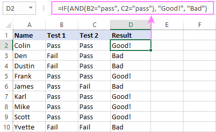
Important note! The AND function checks all the conditions, even if the already tested one(s) evaluated to FALSE. Such behavior is a bit unusual since in most of programming languages, subsequent conditions are not tested if any of the previous tests has returned FALSE.
In practice, a seemingly correct IF statement may result in an error because of this specificity. For example, the below formula would return #DIV/0! ("divide by zero" error) if cell A2 is equal to 0:
=IF(AND(A2<>0, (1/A2)>0.5),"Good", "Bad")
The avoid this, you should use a nested IF function:
=IF(A2<>0, IF((1/A2)>0.5, "Good", "Bad"), "Bad")
For more information, please see IF AND formula in Excel.
Excel IF function with multiple conditions (OR logic)
To do one thing if any condition is met, otherwise do something else, use this combination of the IF and OR functions:
The difference from the IF / AND formula discussed above is that Excel returns TRUE if any of the specified conditions is true.
So, if in the previous formula, we use OR instead of AND:
=IF(OR(B2>50, B2>50), "Pass", "Fail")
Then anyone who has more than 50 points in either exam will get "Pass" in column D. With such conditions, our students have a better chance to pass the final exam (Yvette being particularly unlucky failing by just 1 point :)
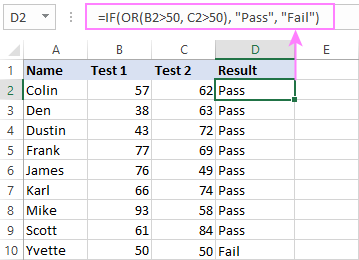
Tip. In case you are creating a multiple IF statement with text and testing a value in one cell with the OR logic (i.e. a cell can be "this" or "that"), then you can build a more compact formula using an array constant.
For example, to mark a sale as "closed" if cell B2 is either "delivered" or "paid", the formula is:
=IF(OR(B2={"delivered", "paid"}), "Closed", "")
More formula examples can be found in Excel IF OR function.
IF with multiple AND & OR statements
If your task requires evaluating several sets of multiple conditions, you will have to utilize both AND & OR functions at a time.
In our sample table, suppose you have the following criteria for checking the exam results:
- Condition 1: exam1>50 and exam2>50
- Condition 2: exam1>40 and exam2>60
If either of the conditions is met, the final exam is deemed passed.
At first sight, the formula seems a little tricky, but in fact it is not! You just express each of the above conditions as an AND statement and nest them in the OR function (since it's not necessary to meet both conditions, either will suffice):
OR(AND(B2>50, C2>50), AND(B2>40, C2>60)
Then, use the OR function for the logical test of IF and supply the desired value_if_true and value_if_false values. As the result, you get the following IF formula with multiple AND / OR conditions:
=IF(OR(AND(B2>50, C2>50), AND(B2>40, C2>60), "Pass", "Fail")
The screenshot below indicates that we've done the formula right:
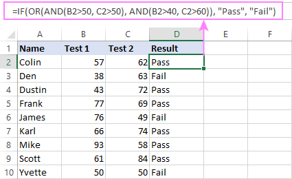
Naturally, you are not limited to using only two AND/OR functions in your IF formulas. You can use as many of them as your business logic requires, provided that:
- In Excel 2007 and higher, you have no more than 255 arguments, and the total length of the IF formula does not exceed 8,192 characters.
- In Excel 2003 and lower, there are no more than 30 arguments, and the total length of your IF formula does not exceed 1,024 characters.
Nested IF statement to check multiple logical tests
If you want to evaluate multiple logical tests within a single formula, then you can nest several functions one into another. Such functions are called nested IF functions. They prove particularly useful when you wish to return different values depending on the logical tests' results.
Here's a typical example: suppose you want to qualify the students' achievements as "Good", "Satisfactory" and "Poor" based on the following scores:
- Good: 60 or more (>=60)
- Satisfactory: between 40 and 60 (>40 and <60)
- Poor: 40 or less (<=40)
Before writing a formula, consider the order of functions you are going to nest. Excel will evaluate the logical tests in the order they appear in the formula. Once a condition evaluates to TRUE, the subsequent conditions are not tested, meaning the formula stops after the first TRUE result.
In our case, the functions are arranged from largest to smallest:
=IF(B2>=60, "Good", IF(B2>40, "Satisfactory", "Poor"))
Naturally, you can nest more functions if needed (up to 64 in modern versions).

For more information, please see How to use multiple nested IF statements in Excel.
Excel IF array formula with multiple conditions
Another way to get an Excel IF to test multiple conditions is by using an array formula.
To evaluate conditions with the AND logic, use the asterisk:
To test conditions with the OR logic, use the plus sign:
To complete an array formula correctly, press the Ctrl + Shift + Enter keys together. In Excel 365 and Excel 2021, this also works as a regular formula due to support for dynamic arrays.
For example, to get "Pass" if both B2 and C2 are greater than 50, the formula is:
=IF((B2>50) * (C2>50), "Pass", "Fail")

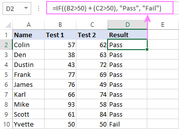
In my Excel 365, a normal formula works just fine (as you can see in the screenshots above). In Excel 2019 and lower, remember to make it an array formula by using the Ctrl + Shift + Enter shortcut.
To evaluate multiple conditions with the OR logic, the formula is:
=IF((B2>50) + (C2>50), "Pass", "Fail")
Using IF together with other functions
This section explains how to use IF in combination with other Excel functions and what benefits this gives to you.
Example 1. If #N/A error in VLOOKUP
When VLOOKUP or other lookup function cannot find something, it returns a #N/A error. To make your tables look nicer, you can return zero, blank, or specific text if #N/A. For this, use this generic formula:
For example:
If #N/A return 0:
If the lookup value in E1 is not found, the formula returns zero.
=IF(ISNA(VLOOKUP(E1, A2:B10, 2,FALSE )), 0, VLOOKUP(E1, A2:B10, 2, FALSE))
If #N/A return blank:
If the lookup value is not found, the formula returns nothing (an empty string).
=IF(ISNA(VLOOKUP(E1, A2:B10, 2,FALSE )), "", VLOOKUP(E1, A2:B10, 2, FALSE))
If #N/A return certain text:
If the lookup value is not found, the formula returns specific text.
=IF(ISNA(VLOOKUP(E1, A2:B10, 2,FALSE )), "Not found", VLOOKUP(E1, A2:B10, 2, FALSE))

For more formula examples, please see VLOOKUP with IF statement in Excel.
Example 2. IF with SUM, AVERAGE, MIN and MAX functions
To sum cell values based on certain criteria, Excel provides the SUMIF and SUMIFS functions.
In some situations, your business logic may require including the SUM function in the logical test of IF. For example, to return different text labels depending on the sum of the values in B2 and C2, the formula is:
=IF(SUM(B2:C2)>130, "Good", IF(SUM(B2:C2)>110, "Satisfactory", "Poor"))
If the sum is greater than 130, the result is "good"; if greater than 110 – "satisfactory', if 110 or lower – "poor".
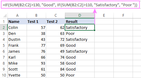
In a similar fashion, you can embed the AVERAGE function in the logical test of IF and return different labels based on the average score:
=IF(AVERAGE(B2:C2)>65, "Good", IF(AVERAGE(B2:C2)>55, "Satisfactory", "Poor"))
Assuming the total score is in column D, you can identify the highest and lowest values with the help of the MAX and MIN functions:
=IF(D2=MAX($D$2:$D$10), "Best result", "")
=IF(D2=MAX($D$2:$D$10), "Best result", "")
To have both labels in one column, nest the above functions one into another:
=IF(D2=MAX($D$2:$D$10), "Best result", IF(D2=MIN($D$2:$D$10), "Worst result", ""))

Likewise, you can use IF together with your custom functions. For example, you can combine it with GetCellColor or GetCellFontColor to return different results based on a cell color.
In addition, Excel provides a number of functions to calculate data based on conditions. For detailed formula examples, please check out the following tutorials:
Example 3. IF with ISNUMBER, ISTEXT and ISBLANK
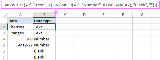
To identify text, numbers and blank cells, Microsoft Excel provides special functions such as ISTEXT, ISNUMBER and ISBLANK. By placing them in the logical tests of three nested IF statements, you can identify all different data types in one go:
=IF(ISTEXT(A2), "Text", IF(ISNUMBER(A2), "Number", IF(ISBLANK(A2), "Blank", "")))
Example 4. IF and CONCATENATE
To output the result of IF and some text into one cell, use the CONCATENATE or CONCAT (in Excel 2016 - 365) and IF functions together. For example:
=CONCATENATE("You performed ", IF(B1>100,"fantastic!", IF(B1>50, "well", "poor")))
=CONCAT("You performed ", IF(B1>100,"fantastic!", IF(B1>50, "well", "poor")))
Looking at the screenshot below, you'll hardly need any explanation of what the formula does:

IF ISERROR / ISNA formula in Excel
The modern versions of Excel have special functions to trap errors and replace them with another calculation or predefined value - IFERROR (in Excel 2007 and later) and IFNA (in Excel 2013 and later). In earlier Excel versions, you can use the IF ISERROR and IF ISNA combinations instead.
The difference is that IFERROR and ISERROR handle all possible Excel errors, including #VALUE!, #N/A, #NAME?, #REF!, #NUM!, #DIV/0!, and #NULL!. While IFNA and ISNA specialize solely in #N/A errors.
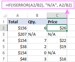
For example, to replace the "divide by zero" error (#DIV/0!) with your custom text, you can use the following formula:
=IF(ISERROR(A2/B2), "N/A", A2/B2)
And that's all I have to say about using the IF function in Excel. I thank you for reading and hope to see you on our blog next week!
Practice workbook for download
Excel IF multiple criteria - examples (.xlsx file)
 by
by
4506 comments
Hi
please am trying to put a formula that would select the best six results out of nine result for an assessment, any help
Hi Eric,
It looks like you need to apply the LARGE function. Please have a look at the following page for more details:
How to get N largest or smallest values
Hope this is what you need.
Please help. I have 1 more argument in this formula need to be incorporated but I don't know how to. This is the formula: =DSUM($A$12:$V$301,"Inv. Amount",$AX$1:$AX$2), where"$A$12:$V$301" is my table for my clients, products they bought and the invoice amount; "Inv. Amount" is the total invoice amount for each client and "$AX$1:$AX$2" is my argument for 1 particular client. Now what I would like to have is highlight one specific product for that particular client. For example I designate "$T$1:$T$2" for product = Basil. Now I like to see ABC company that bought basil, chili,onion...highlight just the amount of basil they bought. I don't know how to incorporate "$T$1:$T$2" into the formula. Thank you in advance for your help.
Tony
Dear,
I am planning to write an if function for 3 criterion.
IF(AND([In Progress - Late]1 >= 1, [At Risk]1 >= 1),[In Progress - On Track]1>=1,) "Red","")
I know I am writing it wrong. Can anyone help me structure the formula?
Cheers!
Dear Michael,
Thank you for contacting us.
For us to be able to help you better, please describe the conditions you have in more detail. It will help us modify your formula to make it work.
Thank you.
Hello,
I am working on project timeline. Client requirement is:
Don't count Sunday & holidays. Now I am facing difficulty when there is a holiday, How I can increase the completion time that was wasted because of that holiday. Formula I used is:
=IF(WEEKDAY(F$3)=1, "holiday",IF(AND(F$3>=$D4,F$3<=$E4),"WORK DAY",""))
Hello, Ibrahim,
If you need to calculate workdays with custom holidays, the NETWORKDAYS function should help you. It returns the number of workdays between two dates, excluding weekends and, optionally, the holidays you specify. If this is what you are looking for, please take a look at this web-page for more details.
If it is not exactly what you need, please specify. We'll do our best to help.
how i can use formoula to caputre data using filter in one sheet to another sheesr. no Material Part HSN / SAC Code Part Price Tax % Model
1 Metal Front Mudguard 87141090 1359.38 28 c-350
2 Metal Cover Tube Black 87141090 311.72 28 c-350
3 Metal Steering Stem (T) 87141090 1359.38 28 c-350
4 Metal Handle Bar 87141090 328.13 28 c-350
5 Metal Air Filter assy 87141090 1025 28 c-350
6 Plastic Trafficator 85122010 211.02 18 c-350
7 Metal Fuel tank 87141090 5846.09 28 c-350
8 Metal Head Lamp 85122010 677.97 18 c-350
9 Metal Front Mudguard 87141090 1054.69 28 Std-350
10 Metal Fual Tank 87141090 6603.13 28 Std-350
11 Metal Frame assy 87141090 6406.25 28 Std-350
12 Metal Air Filter Box 87141090 1275 28 Std-350
13 Metal Cover Resonator 87141090 320.31 28 Std-350
14 Metal Lever and Holder lh 87141090 262.5 28 Std-350
15 Metal foot Rest Arm 87141090 142.19 28 Std-350
16 Metal Swing Arm 87141090 1472.66 28 Std-350
17 Metal Head Lamp Assy 85122010 593.22 18 Std-350
18 Metal Crankcase assy 87141090 11775 28 Std-350
19 Metal Exhaust Pipe (Bend) 87141090 3203.13 28 Std-350
20 Metal front Spindle Kit 87141090 209.38 28 Std-350
21 Metal Tool Box 87141090 1206.25 28 Std-350
22 Metal Saree Gurad 87141090 1038.28 28 Std-350
23 Metal Fork Pipe Spinning 87141090 755.47 28 Std-350
24 Metal Head lamp Casing 87141090 2775.78 28 Std-350
25 Metal Handle Bar 87141090 327.34 28 Std-350
26 Metal Front Mudguard Center stay 87141090 39.06 28 Std-350
27 Metal Silencer Assy 87141090 2416.41 28 Std-350
28 Metal Fuel tank 87141090 7812 28 C-350 Matt
29 Metal Front Mudguard 87141090 1796.88 28 C-350 Matt
i want some date just use filter to another worksheet
Hello, Rohit,
Thank you for contacting us.
I'm sorry but your task is not entirely clear. For us to be able to help you better, please describe it in more detail.
We'll do our best to help.
hi
Good after noon,
I want to show a cell content as debit or credit depending up on previous cell value
Eg: if the cell value is 55 then next cell will shows credit if the cell value is -50 next cell will show debit.Can you please help me to solve this problem.
Syamlal:
Are the only two possibilities "55" and "-50"? If so, then use
=IF(A2=55,"Credit","Debit") where the data is in A2.
If the data is dynamic and is stored in cells A2 and down the column then just copy the formula down the column and it will reflect the results from examining the cells A3, A4, etc.
If the data is dynamic and always shown in the same cell then something like =IF(Cell Address=50,"Credit","Debit").
Or maybe the situation might be If the data in a cell address is less than zero then debit.
There are a number of possibilities for this scenario. You'll have to be more specific with your request to get the answer to your question.
This formula is exactly what i need and i appreciate for sharing.
However with me did not work
I have only one column the Result if less than 28 is Fail if Above 28 is Pass
I went in Manager Formattin Conditional create a rule but it did not give me the Result Pass or Fail
I believe is because i used only one value the médium value of score.
If i6>28 , "pass") other rule
IfI6<28," fail")
If you can help me on this I appreciate. Maria
Hello, Maria.
If you want the cells to be colored automatically depending on the values in column I, please have a look at this article on our blog:
Excel formulas for conditional formatting based on another cell value
However, if you just need a formula to add "pass" or "fail", please try this one:
=IF(I6 >= 28, "pass", "fail")
Please let us know if this is not exactly what you need. We'll do our best to help.
Hello, Jessica:
I think this will work for you:
=IF(COUNTIF(E28:E43,"TRUE"),"Yes","No")
Jessica:
I should add that the "TRUE" value is case sensitive. So, with your data it might be "true".
Hi there,
I need to scan a column of values and get Yes if and only if all the values of the column are equal to a specified value.
E.g. Scan E28:E43 which has a mix of "true" and "false" and return "yes" only if all the values in the range are "true".
Any suggestions on which function I can use?
Thanks!
Jeremy:
If there are only two possible responses for P10 then enter this in S10:
=IF(P10="Yes","Required","check requirements with provider")
I say two responses because in this case No or Unsure are the same response.
Hi there,
I am trying to have a cell automatically fill in a choice of two phrases depending on what the value is in another field.
So, here is what I am trying to achieve:
if P10 = Yes, then I want S10 to say "Required" as well as
if P10 = No or Unsure, then I want S10 to say "check requirements with provider"
=IF(OR(AND(M5>0,M5=4,K5=5,M5=14,K5<20)),0.05769)
Please help! Not sure why I'm getting an error on this. looking to provide an IF statement based on multiple conditions that include an "OR" condition as part of multiple ranges.
Thanks!
=IF(OR(AND(M5>0,M5=4,K5=5,M5=14,K5<20)),0.05769)
Please help! Not sure why I'm getting an error on this. looking to provide an IF statement based on multiple conditions that include an "OR" condition as part of multiple ranges.
Thanks!
Hi,
I have to write if condition based on TEXT vales,Please advise.
i have A,B,C,D,E in one column and in another column i need to get
using if condition that if A,C,E = Yes B,D = NO
I have a condition where i am using three values which return different answers.
RK002-AM
RK002-AD
RK002-AE
RK002-AF
RK002-AG
RK002-AH
RK002-AK
RK002-AL
RK002-AN
RK002-AP
RK002-AR
RK002-AS
RK002-AT
RK002-AU
RK002-AV
RK002-AX
Should return "RTXP8"
RK115-AN
RK115-BF
RK115-AD
RK115-BM
RK115-DF
RK115-BP
RK115-CY
RK115-BB
RK115-CP
RK115-BN
RK115-CM
RK115-DC
RK115-DM
RK115-AK
RK115-DN
RK115-AA
RK115-AB
RK115-AC
RK115-AE
RK115-AF
RK115-AG
RK115-AH
RK115-AL
RK115-AM
RK115-AP
RK115-AR
RK115-AS
RK115-AT
RK115-AU
RK115-AV
RK115-AX
RK115-AY
RK115-AZ
RK115-BA
RK115-BC
RK115-BD
RK115-BE
RK115-BG
RK115-BH
RK115-BK
RK115-BL
RK115-BR
RK115-BS
RK115-BT
RK115-BU
RK115-BV
RK115-BX
RK115-BY
RK115-BZ
RK115-CA
RK115-CB
RK115-CC
RK115-CD
RK115-CE
RK115-CF
RK115-CG
RK115-CH
RK115-CK
RK115-CL
RK115-CN
RK115-CR
RK115-CS
RK115-CT
RK115-CU
RK115-CV
RK115-CX
RK115-CZ
RK115-DA
RK115-DB
RK115-DE
RK115-DG
RK115-DH
RK115-DK
RK115-DL
RK115-DR
RK115-DS
RK115-DT
RK115-DU
RK115-DV
RK115-DX
RK115-DY
RK115-DZ
RK115-EA
RK115-EB
RK115-EC
RK115-ED
RK115-EE
RK115-EF
1MYN565010-D
1MYN565010-E
Should return "RTXP18"
RK315-AM
RK315-BL
RK315-BF
RK315-AA
RK315-AB
RK315-AC
RK315-AD
RK315-AE
RK315-AF
RK315-AG
RK315-AH
RK315-AK
RK315-AL
RK315-AN
RK315-AP
RK315-AR
RK315-AS
RK315-AT
RK315-AU
RK315-AV
RK315-AW
RK315-AX
RK315-AY
RK315-AZ
RK315-BA
RK315-BB
RK315-BC
RK315-BD
RK315-BE
RK315-BG
RK315-BH
RK315-BM
RK315-BN
RK315-BP
RK315-BR
RK315-BT
RK315-BU
RK315-BV
RK315-BX
RK315-BY
RK315-BZ
RK315-CA
RK315-CD
RK315-CG
RK315-CH
RK315-CK
RK315-CL
RK315-CM
RK315-CP
RK315-CR
RK315-CS
RK315-CT
RK315-CU
RK315-CV
RK315-CX
RK315-CY
RK315-CZ
RK315-DA
RK315-DB
RK315-DC
RK315-DD
RK315-DE
RK315-DF
RK315-DG
RK315-DH
RK315-DK
RK315-DL
should Return "RTXP24"
I used the IF conditions and got too many arguments error
APMG xxxxxxx
xxxxxxx
xxxxxxx
xxxxxxx
xxxxxxx
xxxxxxx
AWP xxxxxxx
xxxxxxx
xxxxxxx
BBC xxxxxxx
xxxxxxx
BSM xxxxxxx
xxxxxxx
AS i above statement left side should be the title & right side should be the awards 7 i want to the name to each respective awards of the cell
Hello everyone,
i need help and can someone advice :
we need to check the date of a project OPL, whether it is due , overdue or remain open.
have tried to insert the formula searched from web :
'=IF(ISBLANK(A2),"",IF(A2<TODAY(),"Overdue","") )
it work for 1 criteria condition check. but we need to check 2nd argument and 3rd arguement.
kindly help to refine the correct formula.
thank you very much. Appreciated.
Thanks a lot! Very useful for me.
Hi there,
Could you please help me i have to satisfied multipal condition then formula to be applied on my calculation sheet, condition are as follows:
IF,E=3/5/7 THEN
1) E=3 THEN IF F= ID/OD F=ID THEN (W+H)+29 OR F=OD THEN (W+H)+21
2) E=5 THEN IF F= ID/OD F=ID THEN (W+H)+34 OR F=OD THEN (W+H)+23
3) E=7 THEN IF F= ID/OD F=ID THEN (W+H)+43 OR F=OD THEN (W+H)+25
I need formula to display all matched column heading for the result with two criteria. If $P$1 matches $A$1:$A30 AND $Q$1 matches $B$2:$O$30 THEN MATCHED COLUMN HEADINGS FROM B1:O1 SHOULD APPEAR IN RESULT CELL.
Thank you in advance for the help
Please help me resolve this issue
If A1=A or B then B1=1 else B1=2
Thanks!
When Using nested AND Statement in excel I get error: Find my below statement and help to identify what is wrong?
=IF(AND(E2>=30000000000,F2="CORPORATE","Global Corporate"),IF(AND(E2>=15000000000,F2="CORPRATE","Large Regional"),IF(AND(E2>=3000000000,F2="CORPORATE","Local Corporate"),IF(AND(E2>=2000000000,F2="SME","Large"),IF(AND(E2>=1000000000,F2="SME","Medium"),IF(E2>=500000000,F2="SME","Small"),IF(AND(E2>250000000,F2="SME","Micro"),IF(AND(E2>=100000000,F2="RETAIL","HNI"),IF(AND(E2>=36000000,F2="RETAIL","Afluent"),IF(AND(E2>=12000000,F2="RETAIL","Middle"),"Mass")))))))))
I am trying to automate a daily report template.
Detailed information will be entered into a separate tab with a column for each day of the week.
In the report I want to be able to enter the date and then for the each of the rows to populate based on the information that is in the data tab for that date.
What formula do I need for this?
Pat:
I believe this is what you're looking for.
In C1 enter:
=IF(AND(A1="Dog",B1="Cat"),"Fight","Bark")
Hi
Would be grateful if someone could help.
I need to put text in several cells in colume 1 from a dropdown which I can do.
I then want to put text in several cells in colume 2 from a drop down.
In colume 3 I want text depending on what text is in colume 1 and 2.
Eg if a1 = "dog" then c1 = "bark"/// but if a1 = "dog" and b1 = "cat" then c1 = "fight"
Thanks
Hi,
Need help. How I can make the following statement into excel formula.
if colunm A<=1 then column C is close should be Close within TAT otherwise Close beyond TAT AND if colunm A<=1 then column C is open should Open within TAT otherwise Open beyond TAT
Column A Column B Column C
0 ? Close
2 ? open
I am trying adding a formula whereby if one scores 0 to 39 the other cell displays U, if scores 40 to 49 the other cell displays E, if scores 50 to 59 displays D,, it goes loke that..
Hello, Andrew,
If we understand your task correctly, the formula below should work for you:
=IF(A1 <= 39, "U", IF(A1 <= 49, "E", IF(A1 <= 59, "D", "")))
Please help me to solve this problem.......
If A1=0 then B1=Y and if A1 is not equal 0 then B1=Cell value of A1
Hello, Rakibul,
Please try to enter the following formula in B1:
=IF(A1 = 0, "Y", A1)
Hope this is what you need.
hi - how use a formula in the return value of "IF' function.
eg - if the value is > 500, then (use a formula)else (use another formula)
Regards
Ram Ramajayam
Hi, I need help.
I have a formula that calculates R-G-Y status of the project based on days left to completion (column G)
=IF(G7>=10, "Green", IF(G7>=1, "Yellow", "Red "))
Now I need to add one more condition: only apply this formula to projects "In Progress" in Column F. How can I modify the existing formula to add this condition?
Example:
If status is "in progress" - apply formula
If status is "complete" or "not started" - leave empty
Thanks in advance!
Hi,
How would I go about adding ISNUMBER to this so it also displays no results? I've tried a few different ways but no joy so far.
=IFERROR(INDEX($D$4:$D$950,$G4,COLUMNS($B$4:B4)),"NO RESULTS")
Thanks!
I need a formula in one cell to return results for another set of cells. I have searched for hours now and I'm really not sure I even know how to ask the question. I have a cell labeled Funding Source on Sheet2 and need to pull text from cells F11:F100 in Sheet1. These cells will only contain the text, "Medicaid", "State", or "County". I need the cell in Sheet 2 (Funding Source) to return the results showing if Medicaid, State, or County (or multiple if more than one type is entered) is entered into cells F11:F100 in Sheet1. So if all the cells in Sheet1 have 'Medicaid' entered, the results should only show "Medicaid" in Sheet2 but if 'Medicaid' and 'State' are entered then the results should show "Medicaid and State". I have tried multiple formulas to no avail. Is it even possible to combine the results of numerous cells into one cell?? Any help is appreciated.
Joel:
Text needs to be enclosed in quotes. So, LOM should be "LOM", etc. Also, there needs to be two more closed parentheses at the end of the formula.
I am trying to write a Function that will give a date in a cell depending on what is selected in the adjacent cell. I am using Excel 2013. I have tried the following function
=IF(E2=LOM,D2-120, IF(E2=MSM,D2-90,IF(E2=ARCOM,D2-60,D2-30)
I want the function to display an award due date 30, 60, 90, or 120 days earlier than a stated leave date based on award submitted.
What am I doing wrong?
Sam:
This is an IF Then Else statement and in general they look like this: IF a condition is true THEN perform an operation OTHERWISE perform something ELSE.
So, your situation might look like this:
=IF(A1=3,A1*B1,A1/B1)
how can make condition for example if 3=4 then mulply other wise devide
Sr. No. Particular Amount Code A B C
1 5454423 200 A 200 0 0
2 564564 200 B 0 200 0
3 6546821 300 C 0 0 100
4 648751 100 AB 50 50 0
5 489796 200 BC 0 100 100
6 249736 150 ABC 50 50 50
7 4841 100 AC 50 0 50
8 649489791 600 A How to posible ? Which formula do you have for code.. plz suggest solution
9 23489494 650 B
10 6494964 400 AC
Very helpful thank you!!
Hi, i am struggling with excel formula. In cells a1,b1,c1,d1 have data acc (or) RES (or) REJ. i want to data in cell f1(result) its final row last entered value only display.
Example:
a1 b1 c1 d1 f1
1 res acc acc
2 res res acc acc
3 res res rej rej
4 res res res res res
I need to create a formula where it would only compute an interest, all three cells meet the criteria. Which is, that all three cells are positive numbers. Is that possible?
Hi, i am struggling with excel formula. In cells b1,b2,b3 have data related to cell a1 . B4, b5,b6,b7 has data related to cell a4. Now I want data in cell c3 containing b1/be/be and so on.
Hi all,
I published this a couple of weeks ago, but no-one responded, so posting again, in the hope that someone might be able to help.
I have a deadline date in H3.
I need the formula in O3 to check whether the deadline (H3) has passed today's date. If it has, it then needs to check whether the work has been completed on time (N3), and dependent on the result, display Late or Not Late.
Additionally, I need it to display Late or not Late if a date has not been entered in N3.
If anyone can help, that'd be great.
I am trying to create a formula that will create a
"0" percent of delay when the age equivalent of a test domain is higher then the student's age, i.e. age is 40 months, age equivalent on test domain is 50 months. I also need to show the child's percent of delay in the same formula, i.e. student's age is 40 months, age equivalent on tests is 35 months = 13 percent delay.
Thanks
I am trying to make general comments on students performance if series of column have better or bad mark with distinction, credit, pass or fail. But my formula returns error how can I make better?
=IF(AND(B4>=70,"Distinction", IF(B4>=55,"Credit", IF(B4>=40,"Pass", IF(AND(C4>=70,"Distinction",IF(AND(C4>=55,"Credit",IF(C4>=40,"Pass", IF(AND(D4>=70,"Distinction",IF(D4>=55,"Credit",IF(D4>=40,"Pass", IF(AND(E4>=70,"Distinction",IF(E4>=55,"Credit",IF(E4>=40,"Pass", IF(AND(F4>=70,"Distinction",IF(F4>=55,"Credit",IF(F4>=40,"Pass","Fail"))))))
A B C D E F G
1 1 90 80 70 85 70 Distinction
2 2 72 66 85 90 65 Credit
3 3 70 75 55 63 50 Pass
4 4 34 80 70 39 35 Fail
Hello, Kasozi:
A couple of things. First, the logic used in this formula is going to return an error. For example it says: "B4>=70,"Distinction", IF(B4>=55,"Credit"", etc.
B4 cannot be greater than or equal to 70 and 55. Also the conditions cannot trigger two different returns.
Secondly, I don't think you need to use "AND" for the reason I gave above. The value in B4 cannot be two different conditions to return two different words.
I think I see what you're trying to get at, but I would recommend you read the explanation and then start by using the example shown in the discussion in the article. Start with the simple example and then build the formula from there. Each time you add another condition check to see if it returns an error. If it doesn't add another and so on.
I would like to make the following formula larger (placed in cell J9):
=IF((I9)="poor";"0";IF((I9)="adequate";"1"))
by adding another two factors:
=IF((I9)="poor";"0";IF((I9)="adequate";"1");IF((I9)="good";"2");IF((I9)="excellent";"3"))
But Excel then states that I've entered too many arguments for this function. Does anyone have a solution?
I need to be able to turn the 4 words into a scoring.
Thanks for your help.
try This formula given below
=IF(I9="poor","0",IF(I9="adequate","1",IF(I9="good","2",IF(I9="excellent","3",""))))
I think It's very simple, please try below formula in same Formate ...
=IF(I9=0,"poor",IF(I9=1,"adequate",IF(I9=2,"good",IF(I9=3,"ecellante",IF(I9=4,"very excellatent")))))
Note: Total no of closing bracket is equal to total no of IF used in the formula.
i want creat template for Over time and shift .. can u help me what formula i want use for this case
Shift
A = 8.0
A1= 7.0
B= 10.0
if im key in A at column A.. and column B . must be 8.0.. If im key in A1 at column A.. column B must be 7.0 ...
what formula ? can do like this.. help me please...
hi,
I need help to fix my formula.
I need to highlight queries that has not been finalised as yet.
If it has been finalised(Q5) the highlight cell J5 must be blank.
if the query status (Q5)is "pended", "in progress" or "blank" the highlight cell J5 must reflect TAT expired.
my formula -
If today’s date (BS6) is greater than I5(date TAT expired on) and Q5 (query status) is Finalised then J5 must be blank (test stops) BUT if Q5 (query status)is "blank", "in progress" or "pended" then J5 must reflect TAT Expired.
In A,B,C,D,E, F Row
A1 -1
B1 -2
C1 -3
D1 -5
E1 -10
A2 -5
B2 -10
C2 -30
D2 -40
E2 -50
In second column result is show,
means If i enter 1 in F1 the A1 should be called and displayed Result of A2 (5)
Same for , If i enter 5 in F1 then D1 should be called and displayed result of D2 (40)
Please send the Excel Sheet Formula if anyone konws.
how can match amount and bill no. with a sheet to other sheets AS BELOW :
21-09-2018 Dr Karnataka Bank A/c No. 01 Receipt 120432.00
21-09-2018 Dr Karnataka Bank A/c No. 01 Receipt 179628.00
01-10-2018 Cr SERVICE CHARGES GST Sales PSS 457 379369.87
01-10-2018 Cr SERVICE CHARGES GST Sales PSS 438 183014.00
09-10-2018 Dr Karnataka Bank A/c No. 01 Receipt 145258.00
09-10-2018 Dr Karnataka Bank A/c No. 01 Receipt 150000.00
OTHER SHEET DATA RELATED WITH ABOVE DATA :
31-08-2018 By SECURITY CHARGES Expenses 292 144027.00
New Ref PSS 60 30 Days 145258.00 Cr
New Ref PSS 60 30 Days 1231.00 Dr
31-08-2018 By SECURITY CHARGES Expenses 293 144027.00
New Ref PSS 59 30 Days 145258.00 Cr
New Ref PSS 59 30 Days 1231.00 Dr
21-09-2018 To HDFC BANK - AHURA CENTRE Bank Payment 1469 576108.00
Agst Ref PSS 144 30 Days 144027.00 Dr
KINDLY HELP ME TO COMPARE WITH MULTIPLE SHEETS.
Can someone, please help me in providing a formula. My problem is as below.
I have the following data:
Salary : $2000
PWL2 : $1900
PWL3 : $1950
PWL4 : $2100
Eligibility: ?
If salary is greater than or equal to PWL2 value, Eligibility field should show as "Eligible on PWL2". If salary is greater than or equal to PWL2 and PWL3 value, Eligibility field should show as "Eligible on PWL2 and PWL3". If salary is greater than or equal to PWL2, PWL3 and PWL4 value, Eligibility field should show as "Eligible on PWL2, PWL3 and PWL4". If PWL2, PWL3 and PWL4 values are greater than Salary value, then Eligibility field should show "Not Eligible".
Hello,
I'm looking for an If formula with times and days
If cell is greater than 01:00 and equal to or less than 04:00 return 0.5 (half a day). but if the cell is greater than 04:00 return 1 (1 day).
Is this possible?
The one formula I have used is:
Start Time Finish Time Total Hours Worked Days to claim
12:00 15:00 3:00 0.5
Formula
12:00 15:00 =F11-E11 ???
I would like days to claim to pull back 0.5 if the sum in "Total Hours Worked" is 3.75 or less. Or pull back 1 if it's over 3.75.
I'm guessing the formula would be a "sum if" but I'm not sure how to write it
I'd be grateful for any suggestions please :)
Day Date Name Start Time Finish Time Total Hours Worked Days to claim
Thursday 11/10/2018 Test 9:00 10:00 1:00
1
Friday 12/10/2018 Test 2 17:00 22:00 5:00
1
Saturday 13/10/2018 Test 3 7:00 22:00 15:00
1
Example formula:
=IF(G22>3.75,"0.5",IF(G22<3.75,"1"))
G22 is the total hours (i.e.1, 5, 15). 1 should pull back 0.5. 5 and 15 should pull back 1
but this formula is not working properly.
I would be grateful if you could please help me fix the formula
Since you want 3.75 or less = 0.5, you should start the equation with > 3.75. Else, excel will read 3.75 as 1.
The basic if equation is like this:
=if(condition, result if condition is met, result is condition isn't met)
So the equation should be like this
= if(A2>3.75,1,0.5)
With A2= working hours
Note: you only need " " if the option are non numerical.