The tutorial shows how to create multiple IF statements in Excel with AND as well as OR logic. Also, you will learn how to use IF together with other Excel functions.
In the first part of our Excel IF tutorial, we looked at how to construct a simple IF statement with one condition for text, numbers, dates, blanks and non-blanks. For powerful data analysis, however, you may often need to evaluate multiple conditions at a time. The below formula examples will show you the most effective ways to do this.
How to use IF function with multiple conditions
In essence, there are two types of the IF formula with multiple criteria based on the AND / OR logic. Consequently, in the logical test of your IF formula, you should use one of these functions:
- AND function - returns TRUE if all the conditions are met; FALSE otherwise.
- OR function - returns TRUE if any single condition is met; FALSE otherwise.
To better illustrate the point, let's investigate some real-life formulas examples.
Excel IF statement with multiple conditions (AND logic)
The generic formula of Excel IF with two or more conditions is this:
Translated into a human language, the formula says: If condition 1 is true AND condition 2 is true, return value_if_true; else return value_if_false.
Suppose you have a table listing the scores of two tests in columns B and C. To pass the final exam, a student must have both scores greater than 50.
For the logical test, you use the following AND statement: AND(B2>50, C2>50)
If both conditions are true, the formula will return "Pass"; if any condition is false - "Fail".
=IF(AND(B2>50, B2>50), "Pass", "Fail")
Easy, isn't it? The screenshot below proves that our Excel IF /AND formula works right:

In a similar manner, you can use the Excel IF function with multiple text conditions.
For instance, to output "Good" if both B2 and C2 are greater than 50, "Bad" otherwise, the formula is:
=IF(AND(B2="pass", C2="pass"), "Good!", "Bad")
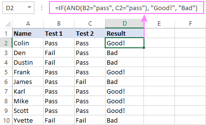
Important note! The AND function checks all the conditions, even if the already tested one(s) evaluated to FALSE. Such behavior is a bit unusual since in most of programming languages, subsequent conditions are not tested if any of the previous tests has returned FALSE.
In practice, a seemingly correct IF statement may result in an error because of this specificity. For example, the below formula would return #DIV/0! ("divide by zero" error) if cell A2 is equal to 0:
=IF(AND(A2<>0, (1/A2)>0.5),"Good", "Bad")
The avoid this, you should use a nested IF function:
=IF(A2<>0, IF((1/A2)>0.5, "Good", "Bad"), "Bad")
For more information, please see IF AND formula in Excel.
Excel IF function with multiple conditions (OR logic)
To do one thing if any condition is met, otherwise do something else, use this combination of the IF and OR functions:
The difference from the IF / AND formula discussed above is that Excel returns TRUE if any of the specified conditions is true.
So, if in the previous formula, we use OR instead of AND:
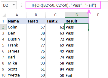
=IF(OR(B2>50, B2>50), "Pass", "Fail")
Then anyone who has more than 50 points in either exam will get "Pass" in column D. With such conditions, our students have a better chance to pass the final exam (Yvette being particularly unlucky failing by just 1 point :)
Tip. In case you are creating a multiple IF statement with text and testing a value in one cell with the OR logic (i.e. a cell can be "this" or "that"), then you can build a more compact formula using an array constant.
For example, to mark a sale as "closed" if cell B2 is either "delivered" or "paid", the formula is:
=IF(OR(B2={"delivered", "paid"}), "Closed", "")
More formula examples can be found in Excel IF OR function.
IF with multiple AND & OR statements
If your task requires evaluating several sets of multiple conditions, you will have to utilize both AND & OR functions at a time.
In our sample table, suppose you have the following criteria for checking the exam results:
- Condition 1: exam1>50 and exam2>50
- Condition 2: exam1>40 and exam2>60
If either of the conditions is met, the final exam is deemed passed.
At first sight, the formula seems a little tricky, but in fact it is not! You just express each of the above conditions as an AND statement and nest them in the OR function (since it's not necessary to meet both conditions, either will suffice):
OR(AND(B2>50, C2>50), AND(B2>40, C2>60)
Then, use the OR function for the logical test of IF and supply the desired value_if_true and value_if_false values. As the result, you get the following IF formula with multiple AND / OR conditions:
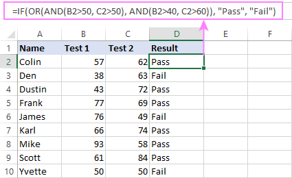
=IF(OR(AND(B2>50, C2>50), AND(B2>40, C2>60), "Pass", "Fail")
The screenshot below indicates that we've done the formula right:
Naturally, you are not limited to using only two AND/OR functions in your IF formulas. You can use as many of them as your business logic requires, provided that:
- In Excel 2007 and higher, you have no more than 255 arguments, and the total length of the IF formula does not exceed 8,192 characters.
- In Excel 2003 and lower, there are no more than 30 arguments, and the total length of your IF formula does not exceed 1,024 characters.
Nested IF statement to check multiple logical tests
If you want to evaluate multiple logical tests within a single formula, then you can nest several functions one into another. Such functions are called nested IF functions. They prove particularly useful when you wish to return different values depending on the logical tests' results.
Here's a typical example: suppose you want to qualify the students' achievements as "Good", "Satisfactory" and "Poor" based on the following scores:
- Good: 60 or more (>=60)
- Satisfactory: between 40 and 60 (>40 and <60)
- Poor: 40 or less (<=40)
Before writing a formula, consider the order of functions you are going to nest. Excel will evaluate the logical tests in the order they appear in the formula. Once a condition evaluates to TRUE, the subsequent conditions are not tested, meaning the formula stops after the first TRUE result.
In our case, the functions are arranged from largest to smallest:
=IF(B2>=60, "Good", IF(B2>40, "Satisfactory", "Poor"))
Naturally, you can nest more functions if needed (up to 64 in modern versions).

For more information, please see How to use multiple nested IF statements in Excel.
Excel IF array formula with multiple conditions
Another way to get an Excel IF to test multiple conditions is by using an array formula.
To evaluate conditions with the AND logic, use the asterisk:
To test conditions with the OR logic, use the plus sign:
To complete an array formula correctly, press the Ctrl + Shift + Enter keys together. In Excel 365 and Excel 2021, this also works as a regular formula due to support for dynamic arrays.
For example, to get "Pass" if both B2 and C2 are greater than 50, the formula is:
=IF((B2>50) * (C2>50), "Pass", "Fail")

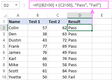
In my Excel 365, a normal formula works just fine (as you can see in the screenshots above). In Excel 2019 and lower, remember to make it an array formula by using the Ctrl + Shift + Enter shortcut.
To evaluate multiple conditions with the OR logic, the formula is:
=IF((B2>50) + (C2>50), "Pass", "Fail")
Using IF together with other functions
This section explains how to use IF in combination with other Excel functions and what benefits this gives to you.
Example 1. If #N/A error in VLOOKUP
When VLOOKUP or other lookup function cannot find something, it returns a #N/A error. To make your tables look nicer, you can return zero, blank, or specific text if #N/A. For this, use this generic formula:
For example:
If #N/A return 0:
If the lookup value in E1 is not found, the formula returns zero.
=IF(ISNA(VLOOKUP(E1, A2:B10, 2,FALSE )), 0, VLOOKUP(E1, A2:B10, 2, FALSE))
If #N/A return blank:
If the lookup value is not found, the formula returns nothing (an empty string).
=IF(ISNA(VLOOKUP(E1, A2:B10, 2,FALSE )), "", VLOOKUP(E1, A2:B10, 2, FALSE))
If #N/A return certain text:
If the lookup value is not found, the formula returns specific text.
=IF(ISNA(VLOOKUP(E1, A2:B10, 2,FALSE )), "Not found", VLOOKUP(E1, A2:B10, 2, FALSE))

For more formula examples, please see VLOOKUP with IF statement in Excel.
Example 2. IF with SUM, AVERAGE, MIN and MAX functions
To sum cell values based on certain criteria, Excel provides the SUMIF and SUMIFS functions.
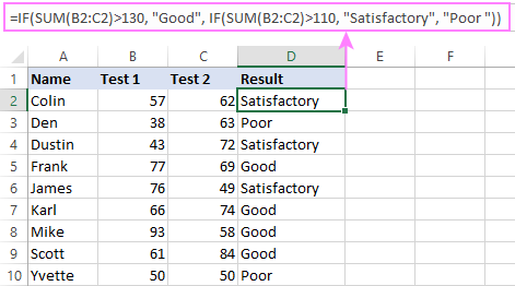
In some situations, your business logic may require including the SUM function in the logical test of IF. For example, to return different text labels depending on the sum of the values in B2 and C2, the formula is:
=IF(SUM(B2:C2)>130, "Good", IF(SUM(B2:C2)>110, "Satisfactory", "Poor"))
If the sum is greater than 130, the result is "good"; if greater than 110 – "satisfactory', if 110 or lower – "poor".
In a similar fashion, you can embed the AVERAGE function in the logical test of IF and return different labels based on the average score:
=IF(AVERAGE(B2:C2)>65, "Good", IF(AVERAGE(B2:C2)>55, "Satisfactory", "Poor"))
Assuming the total score is in column D, you can identify the highest and lowest values with the help of the MAX and MIN functions:
=IF(D2=MAX($D$2:$D$10), "Best result", "")
=IF(D2=MAX($D$2:$D$10), "Best result", "")
To have both labels in one column, nest the above functions one into another:
=IF(D2=MAX($D$2:$D$10), "Best result", IF(D2=MIN($D$2:$D$10), "Worst result", ""))

Likewise, you can use IF together with your custom functions. For example, you can combine it with GetCellColor or GetCellFontColor to return different results based on a cell color.
In addition, Excel provides a number of functions to calculate data based on conditions. For detailed formula examples, please check out the following tutorials:
Example 3. IF with ISNUMBER, ISTEXT and ISBLANK
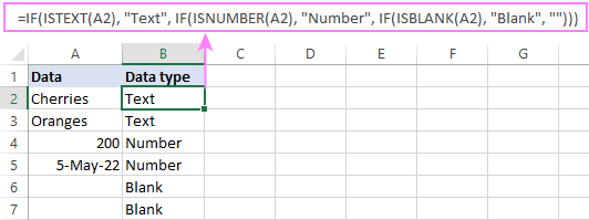
To identify text, numbers and blank cells, Microsoft Excel provides special functions such as ISTEXT, ISNUMBER and ISBLANK. By placing them in the logical tests of three nested IF statements, you can identify all different data types in one go:
=IF(ISTEXT(A2), "Text", IF(ISNUMBER(A2), "Number", IF(ISBLANK(A2), "Blank", "")))
Example 4. IF and CONCATENATE
To output the result of IF and some text into one cell, use the CONCATENATE or CONCAT (in Excel 2016 - 365) and IF functions together. For example:
=CONCATENATE("You performed ", IF(B1>100,"fantastic!", IF(B1>50, "well", "poor")))
=CONCAT("You performed ", IF(B1>100,"fantastic!", IF(B1>50, "well", "poor")))
Looking at the screenshot below, you'll hardly need any explanation of what the formula does:

IF ISERROR / ISNA formula in Excel
The modern versions of Excel have special functions to trap errors and replace them with another calculation or predefined value - IFERROR (in Excel 2007 and later) and IFNA (in Excel 2013 and later). In earlier Excel versions, you can use the IF ISERROR and IF ISNA combinations instead.
The difference is that IFERROR and ISERROR handle all possible Excel errors, including #VALUE!, #N/A, #NAME?, #REF!, #NUM!, #DIV/0!, and #NULL!. While IFNA and ISNA specialize solely in #N/A errors.
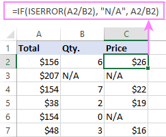
For example, to replace the "divide by zero" error (#DIV/0!) with your custom text, you can use the following formula:
=IF(ISERROR(A2/B2), "N/A", A2/B2)
And that's all I have to say about using the IF function in Excel. I thank you for reading and hope to see you on our blog next week!
Practice workbook for download
Excel IF multiple criteria - examples (.xlsx file)
 by
by
4506 comments
So glad I have found this! But need help with a multiple condition IF and AND formula.
If Column C = regular, column D= technician, result is 97.5 but how to add if Column C or D is something different to change the result?
=IF(((AND(C2:C25="REGULAR",D2:D25="TECHNICIAN")),97.5)'c2:c25="priority",d2:d25="technician", 146.25)
I am looking at using 6 different results/combinations.
Hi everyone,
I really need your help. The table below represents opportunities and its value for each prospect as follows;
Prospect I Value I Stage
------------------I----------------------------------
Company A I $2000 I Stage 1
Company B I $3000 I Stage 2
Company C I $1000 I Stage 1
Company D I $2000 I Stage 1
Company A I $3000 I Stage 2
Company B I $5000 I Stage 3
Company A I $7000 I Stage 4
Company C I $3000 I Stage 3
1. I wanted to show ONLY the last value of the last stage for each company
Company I Value I Stage
------------------I--------------------I---------------
Company A I $7000 I Stage 4
Company B I $5000 I Stage 3
Company C I $3000 I Stage 3
Company D I $2000 I Stage 1
2. I wanted to Add those last value of the last stage to have;
Stage 1 I Stage 2 I Stage 3 I Stage 4
---------------I------------------I------------------I----------------
$2000 I $0 I $8000 I $7000
I would really appreciate any feedback even on one of the two parts.
Hello,
I'm confusing to use If And or IF Or function for following issue.
If the on hand stock of each Size 6, 7 and 8 is zero, i would like to appear it as "size broken" and If the on hand stock of the rest size 5 and 9 is zero, it's nothing to appear.
For example - I used below function but it does not work.
IF(AND(C7=7,8,9,D7<=0),"Size broken","")
Any help would be appreciated.
HI
i need guidance regarding following problem.
I have data in three columns,First column contain ID, Second contain Disease name and third also contain disease name, now one ID is in multiple rows with data, so how can i combine data of same IDs in one row, and then in one cell.
Thanks
Hi Asim,
If we understand your task correctly, our Merge Duplicates Wizard can help you with this task. It allows you to combine duplicate rows into one without losing any data.
Hi there! I have a formula that could be pretty long. Looking for some help.
If column E = Eagle and column D = Select 6 and column P = 0-75 then column Q = 1.5%
If column E = Eagle and column D = Select 6 and column P = 76-80 then column Q = 1.1%
If column E = Eagle and column D = Select 6 and column P = 81-85 then column Q = .75%
If column E = Eagle and column D = Platinum 5 or Platinum 7 and column P = 0-75 then column Q = .75%
If column E = Eagle and column D = Platinum 5 or Platinum 7 and column P = 76-80 then column Q = .50%
If column E = Eagle and column D = Platinum 5 or Platinum 7 and column P = 81-85 then column Q = .38%
If column E = Symetra and column D = Edge GPS 5 or Edge GPS 7 then column Q = 1%
If column E = Symetra and column D = Advantage Income, Custom 5, Custom 7, Select 5 or Select 7 then column Q = .5%
Hi, i am entering multiple values separated by comma in a single cell and i do not want two values (for ex. a and b) to come together in a single cell. can you please tell the formula?
=IF(AND(E9>=75,F9=75,F9<11),E9*2%,0)
I need ur help to create right formula. This is giving results but not in numbers
Hi,
I'm very new to Excel and i'm trying to achieve something I was told is possible but I have no idea how.
I'm after a formula that will return a value in one cell depending upon the data in another cell.
For example;
I want cell C2 to display 'PB' if any of 15 school names are typed into A2, 'FL' if a any of 5 names are typed in A2, 'EC' = 6 names in A2, 'RT' = 4 names, 'SK' = 13 names, 'SH' = 8 names, 'KL/WN' = 8 names and 'Hunt' = 7 names.
I've tried nesting If functions and IF/OR, but I just receive errors saying there are too many arguments.
Here is a quick snippet of a shorter version I tried; =IF(OR($A2="Abbey College",$A2="Ernulf Academy"),"Hunt","",IF(OR($A2="Jack Hunt",$A2="AMVC"),"PB",""))
Any help would be appreciated.
Thanks,
Name Math Physics Chemistry English Total Average Status No. of Paper Fails Name of Failed Subjects Fine
a 35 23 14 65 102 34 Fail 2 Physics 400
b 0 45 34 74 153 51 Pass 0 0
c 0 43 44 36 123 41 Pass 0 72
Passing marks are 33 and i want to have name of subjects failed by the student in one column
HI
i need guidance regarding following problem.
I have data in three columns,First column contain ID, Second contain Disease name and third also contain disease name, now one ID is in multiple rows with data, so how can i combine data of same IDs in one row, and then in one cell.
Thanks
=If(c1="a","aa",if( c1="b","bb.... continue more than 64 serially but not success after 64 times so if anyone know please help me.
Help i want a conditional format that basically does the below
To be calculates in N4.......if L4 States External then N4 will x100 then / 12. Producing the final figure in G4
i am really confusing myself trying to do this on a sheet basically ionly want a cell to wor ot the percentage of a salary if it deemed as external
Help
Hi,
I input an amount of items into my spreadsheet in either column D or column E - never both. I then input a price into column F (for info - if under 6 are ordered then sale price is 0.57, over 6 and price is 0.55).
I am looking for a formula which can multiply column F (my price) by either column D or E (my amount of items) and give me an overall price but I want the formula to be able to 'know' which column to 'pick' given on which one has data entered into it; any ideas?
Many Thanks,
Hi I have tried multiple IF formula but can't get it to work. I want to show a number in cell A2 (5, 10, 15, 30) depending on a percentage in cell A1 (>=102%, >=110%, >=125%, >=150%)
>=102%=5
>=110%=10
>=125%=15
>=150%=30
thanks for any help
Customer Type drs order unit rate total add total
Farmer 1 unit apple 1 30 30 30 60
c2f 1 unit apple 1 30 30 0 30
Farmer 1 unit apple 1 unit orange 1 30 30 0 30
Farmer 1 unit apple 1 30 30 30 60
c2f 1 unit apple 1 30 30 0 30
Farmer 1 unit apple 1 unit orange 1 30 30 0 30
i need advice
if cell contain farmer with 1 qty charge him 30 rs
if cell contain c2f with 1 qty then dont charge 30 rs
if cell contain more then 1 product then also don't charge any thing but highlight the cell with colour
pls advice
I am struggling with a formula. I'm in Accounts Receivable and I'm comparing invoiced quantities, prices and amounts to what was paid. I'll put this vertically due to lack of horizontal room in this comment box.
Column M = Invoiced Qty
Column N = Invoiced Price
Column O = Amount Invoiced
Column P = Paid Qty
Column Q = Paid Price
Column R = Paid Amount
Column S = Difference (Sum of O-R)
So, I want in column T to be:
"Q" if there is a difference between Column M and Column P,
"P" if there is a difference between Column N and Column Q,
"QP" if there is a difference between both Columns M & P AND N & Q,
"NP" if there are blanks in Columns P & Q (maybe it would be easier to say if Column O = Column S), or
to be blank if none of these conditions are met.
Can you help? I've tried several methods and I can always get it to do some of these but not all conditions.
Thank you!
I AM FACING A PROBLEM AND GUIDANCE IS NEEDED?
THERE ARE TWO SUBJECTS IN A1 AND B1
ENGLISH READER IN A1 AND ENGLISH GRAMMAR IN B1
EACH SUBJECT CARRIES 100 MARKS EACH.
MINIMUM PASSING MARKS ARE 35% OR 35 MARKS.
NOW TO CREATE RESULT FOR ENGLISH IS
ENGLISH = ENGLISH READER MARKS + ENGLISH GRAMMAR MARKS.
NOW ONLY THOSE MARKS WILL BE COUNTED WHICH IS AT LEAST 35 PERCENT.
A1= 34 B1 = 35
ENGLISH = A1 + B1 =35
A1 MARKS WILL NOT BE COUNTED SINCE AT LEAST 35 MARKS NEEDED TO ADD.
IF A1 = 35 AND B1=35 THEN
ENGLISH TOTAL MARKS WILL BE = A1+B1=35+35=70
BUT SINCE A1 HAS34 VALUE THEN
ENGLISH TOTAL MARKS SHOULD BE = A1(0)+B1(35)=35
PLEASE HELP TO GET OUT THIS CONFUSING SITUATION....
WHAT TYPE OF FORMULA SHOULD BE THERE....PLEASE MENTION.
THANKS.
what is the formula to create a grouping such as below
a= 0>
what will be the syntax to formulate data below for the given conditions
>0 & 90 & 180 & 270 & 365 = e
Age Days
43
334
350
334
233
242
248
250
280
16
82
113
82
113
93
93
113
Hello,
What is the formula to get an output of below given situations:
A1 = DEF OR is blank
B1 = ABC
C1 = AAAA
RESULT D1 = DEFAAAA (if A1 have text) OR ABCAAAA (if A1 is blank)
help please
Column A1 = 10
Coumn B1 = 4
Column A1 will become 6
then if user input another value in B1 it will deduct again from A1
I want to create such a formula where if the completion date say 16.05.2018 is less than 28.05.2018 than i want the amount to be displayed otherwise zero. In the excel sheet date will also vary after 4 -5 batch and in between amount could also be different. Please someone help.
Hi Friends please advise?
i need formula for this, i have 96 value but need to multiply between (1-50)*50+(51+75)*75+(76+till the end value)*100=====
please fix the formula and advise my, great thanks.
Hi Friends please advise?
i need formula for this, i have 96 value but need to multiply between (1-50)*50+(51+75)*75+(76+till the end value)*100=====
please fix the formula and advise my, great thanks.
I am fighting a formula in Excel involving loan amortizations. Long story short, I am wanting to show nothing in cell G17 if J16 has a zero balance. If it does have a balance, I want the result to be the value in D5 to be shown in G17. These are samples of what I've tried:
=IF(J16=0,"",IF(J160,-$D$5)) . . . the value of D5 still shows.
=IF(J160,-$D$5),IF(J16=0,"") . . . the result is #VALUE!
Any help would be appreciated. Thanks.
If i press 1 then next cell value is 18000-56900,
If i press 2 then next cell value is 19900-63200,
If i press 3 then next cell value is 21700-69100,
If i press 4 then next cell value is 25500-81100,
My question is how is it possible to arrange in excel formula to get correct value of each number. please tell me with example.
Hi,
Svetlana
Can you please assist me, the same cell if a positive value should be 'Dr' if negative should be 'Cr'
=IF((AND(G5>=0.1,G5<0.1)),"Cr","Dr")
Hi!
I think you've overthought it :)
=IF(G5>=0.1,"Cr","Dr")
=IF(A9>=5.28,A9-5.28,A9/0.033,IF(A9>=10.08,A9-10.08,A9/0.072))
Hi,
I am trying to create a point system with below numbers. How do I use this formula. There are different criteria's for each column.
Eg: If someone get Yes's it is positive and they get No it will be negative scores. Also, other two things need to give some range say from 10.00 to 13.00 = 3 scores, if it is less than 9.99 should get 4 scores. I would appreciate your help.
Hi, Could someone help me to create a formula for:\
"IF D1 = A2 return the value in B2 or IF D1=A2 return the minus value in C2
Thank you!
regards
Not sure what you are asking unless you want B2 or C2 to be returned as the If False condition.
If D1=A2 the formula will either return B2 or C2, but not both.
Try this and see if it works for you: =IF(D1=A2,B2,C2)
If the value in D1 is equal to the value in A2 then return the value in B2 otherwise return the value in C2.
Value to Org. Impact on Org.
Value - Value Text Option Value - Impact Text Options
Column x - Column y Column z - Column aa
0 Not Important 0 No impact
1 Low importance 1 Low impact
2 Medium importance 2 Medium impact
3 High importance 3 High impact
4 Very high importance 4 Very high impact
I have put Value text in drop down in one cell and Impact Test Option in right side Box
There can be any combination of Value Text and Impact Text - Based on the selected text, the respective value of both Values have to be put on right adjust box
Example - For Low Importance & Low impact
I have put the formula as =IF(C6=Y2, D6=AA2,X2*Z2) i am getting result as under:
Organization Impact Factor Reputation Impact Factor Criticality
Low importance Low impact "TRUE" instead of requirement as:
Low importance Low impact 1 (as Value for Low importance is 1 & Low Impact is 1 - so 1x1=1)
Please help me with the formula so that I get 1 as answer?
I'm working on a budgeting sheet and need a formula that only adds/subtracts transactions IF there is a certain word typed in the category cell (i.e. "Grocery"), but won't include other categories I put in (i.e. "Rent" or leaving it blank).
So far I have:
=IF(D4="Grocery",L3-F4+G4,L3)
It works, but only for one transaction. I need it to cover the whole sheet somehow to get an accurate total for each "budget" category. [I have a transaction side of the sheet and then a "budget" side with the categories and their totals (i.e. "Grocery" in one cell and "$50" next to it as the total). The "$50" is the cell I'm placing the formula in.]
Hi Svetlana,
I'm trying to do an inventory management sheet and need to calculate totals of certain items. So in cell 1 we can use "Plugable", for cell 2 we can use a quantity like "1" and then in cell three, if the item is "in", "out" or "damaged", in cell 4, the total of how many Plugables are being used. I'm not sure how to do that.
So 4 cells and a running total of how many are "in", "out" or "damaged".
I have some queries for you as belows:-
Is it possible to create excel Sales Report of a particular employee among multiple employees with FOUR different conditions: (1) Specific Date / Period Wise, (2) Employee Wise, (3) Multiple Region Wise & (4) Multiple Product Wise
Example: How much "Laptop" and "Desktop" and "UPS" and "Keyboard" (i.e. the Products) INDIVIDUALLY sold by "Mr. Ankit" and by "Mr. Rocky" and by "Mr. Samir" and by "Mr. Karan" (i.e. the Employees) in the Region "North" and "South" and "East" and "West" for any specific period of last 1 or 2 or 3 Years OR Months OR Quarters OR Days
Further Conditions:-
1) No VBA requires
2) Only Excel 2007 and below formulas / functions has to be used
how to Caluclated Dr is +, cr is -
DR 10
CR 20
DR 20
Hello there,
If I understand your task correctly and you'd like to turn numbers for CR to negative and your data are in columns A and B, the following formula should do for column C:
=IF(A1="DR",B1,-(B1))
Can someone help, need an excel formula.
I have two columns.
Column A contains dates (just month and date) i.e. September 09
Column B contains texts either "Complete" or No"
I want to compare cell A1 if it contains a date to Cell B1 if it contains text and give results "Done" or " Not done"
Results: If cell A1 = date and cell B1 = text complete then "Done"
If cell A1 = no date and B1 = text completed, then "Not Done"
Sofy:
There are a couple of ways to accomplish what you want to do. Here is one that doesn't require VBA.
=IF(AND(CELL("Format",D24)="D2",E24="Complete"),"Done","Not Done")
Where the date is in D24 and it is in the dd/mmm as in your sample.
Where "Complete" is in E24 enter this formula in an empty cell.
So, it says, if the format of the contents of cell D24 is a date in the format 9-September and the contents of E24 is "Complete" then display "Done" otherwise if one or both of these are not true display "Not Done".
Hi,
PLEASE HELP ME TO FIND THE BELOW NO. IS IN BETWEEN 5 & 10 USING IF FORMULA
8
A B C D E ANSWER
DATE OF JOIN CURRENT DATE BASIC DA
1 01-01-2010 22-12-2018 8,000.00 2,340.00 517
DATEDIF(B4,C4,"y") = 8
IF(AND(DATEDIF(B4,C4,"y")<5,(DATEDIF(B4,C4,"y")<10)),(D4+E4)*0%,(D4+E4)*5%)
A B C D E ANSWER
DATE OF JOIN CURRENT DATE BASIC DA
2 01-01-2015 22-12-2018 8,000.00 2,340.00 0
DATEDIF(B4,C4,"y") = 3
IF(AND(DATEDIF(B6,C6,"y")<5,(DATEDIF(B6,C6,"y")10,(D8+E8)*10%,(D8+E8)*5% )
WHAT'S THE SYNTAX FOR THESE 3 IF CONDITIONS IN ONE EQUATION
1) IF C5 10 =10%
Hi,
I need help with an "if,then" statement. I want to say the following:
If C3 is 50% of B3, then D3 should be 0.
If C3 is not 50% of B3, then D3 should be 50% of C3
Hi Donterrio,
Here's the formula for B3:
=IF(C3=B3*0.5, 0, C3*0.5)
HI Svetlana!
I am trying to come up with an excel formula for the following:
Up to $ 50,000.00 $ 850.00
$ 50,001.00 To $ 150,000.00 $ 1025.00
$ 151,001.00 To $ 200,000.00 $ 1100.00
$ 200,001.00 To $ 250,000.00 $ 1175.00
$ 250,001.00 To $ 300,000.00 $ 1250.00
$300,001.00 To $ 350,000.00 $ 1325.00
$ 350,001.00 To $ 400,000.00 $ 1,400.00
$400,001.00 To $ 500,000.00 $ 1,550.00
$500,001.00 To $ 750,000.00 $ 1800.00
$750,001.00 & UP $ 2100.00
does any know how to sort/filter data by x,y coordinates?
here is the situation:
i am pulling map data by zip code and putting it into a csv file. enclosed inside these zip codes are
distribution areas. i have 4 lat/lons (x1,y1), (x2,y2), (x3,y3), and (x4,y4) these create a square geographic boundary that is a DA. what i would like to do is filter out the data that is not enclosed in the boundary.
I can do this in matlab however, my company does not own matlab so i am attempting to do this in excel. please help if you can
Hello Svetlana,
I have to write a formula for the following condition:
Application filled by students are saved in an excel file where there are fields where students enter which class they study in and the subjects they opt for. Now I have the columns to enter the class (from a drop-down list) and SUBJECTS OPTED (multiple selection dropdown lists). Now based on the values entered I need to get a result as to the total fees they need to pay called from another sheet.
How do I do that (tried with no success)?
Kindly Help.
Can Anyone rectify my below formula.
Instead of Result, it shows me as #VALUE!
=IF(K3=0,"Nil",TODAY()-C3)*AND(IF(K3>0,"Excess",TODAY()-C3))*AND(IF(K3<0,TODAY()-C3,"Bal"))
Hi there. I am trying to produce a formula for the following:
IF A1 contains Receivables, copy b1 as a positive number in c1.
Any ideas?
Hi Casey,
Here's the formula for C1:
=IF(A1="Receivables", ABS(B1), "")
Thank you! Youre a wiz! One more question: The word receivables is in a sting of words in A1. How do I write this into the formula?
Hi Casey,
In this case, you can use the SEARCH function to find it :)
=IFERROR(IF(SEARCH("receivables",A1), ABS(B1)), "")
great article -thank you!
I am stumped on one that I would love your expert opinion on....I want to combine and AND with a formula, so basically if cell E3>0 then H2*E3 (I have to cost out the cost of an employee to fly out for a certain travel day, but only of that travel day is required. By placing a 1 in cell E3 I am saying that we need a travel day, so want it to activate the formula H2*E3).
Know this is complicated but thank you for reading this one anyway!
OK, I'll bite.
=IF(E3>0,H2*E3,"Stumped")
Thank you Doug!
Help, I need to make a formula for cells for the following. If between 2-5 then 1, If between 6-10 then 2 and so on. Please help
1 first aid attendant for 2-5 employees per floor at all times
2 first aid attendants for 6-10 employees per floor at all times
3 first aid attendants for 11-50 employees per floor at all times
4 first aid attendants for 51-100 employees per floor at all times
5 first aid attendants for 101-150 employees per floor at all times
6 first aid attendants for 151-200 employees per floor at all times
Hello, Rhea,
If we understand your task correctly, the following formula should work for you:
=IF(A1 >= 151, 6, IF(A1 >= 101, 5,IF(A1 >= 51, 4, IF(A1 >= 11, 3, IF(A1 >= 6, 2, IF(A1 >= 2, 1, ""))))))
Hello,
I am searching for a function that first is searching on a column for 11.75 with fill color white, and on the line that find this is searching in another area for X, and if this is true put X or 1 or something in that cell.
I put here a file with this if I didn't explain that well:
https://docs.google.com/spreadsheets/d/1_mEK7awCtL06UiAmPEE1hZ3u1_Dj0j1eyoWAPB4s44U/edit#gid=0
Can anyone help me with this formula?
Cheers!
Hi, Daniel,
We've looked into your task and have a couple of questions to clarify before we can help:
1) Since you posted your question under the article about Excel - do you need a solution for Excel or Google Sheets? These platforms work a bit differently, so we need to know for sure.
2) You mentioned you need to put "X" instead of "11.75" when the latter occurs. I'm afraid it won't be possible, because the formula returns the result to where it stands, and we can't enter it to the cell needed for the calculations.
3) Could you please also clarify where is the "day" in your data? It's not entirely clear whether the days are the columns from A to E, or the ranges like A21:E25.
You can email us to support@ablebits.com with the answers for better convenience.
Thank you.
I am trying to write a formula for the below scenario:
We have a list of data entered by our customer service reps (CSRs). Each day, we need to know if the specific members of our pilot group were there.
I have a table with a row at the end labeled 1-5 (for days of the week).
I'm trying to develop a formula that will look for Day 1 (or Day 2, etc.) and then look through the list of names (which will actually include all 5 days) and return a value of "Yes" or "No".
I've got a whole Word document of attempted formulas and nothing is working. I thought this would work (I created additional tabs for days and the pilot group names):
=IF((AND('Qry_BCNA Control Group'!$O:$O='Days '!$A$1, 'Qry_BCNA Control Group'!$K:$K='PilotGroup'!$A:$A)), “Yes”, “No”)
But it came back with a #NAME? error.
I have 8 partners in company. 3 of them are silent they have invested, 2 of them are active but not invested, and remaining 3 are both active and also invested. I want to give them different margin share of the profit. I want to give silent partners 20% of the profit amount, active 30%, and 50% to the active and investors.
1. partner1= 0 eqity active
2. partner2= 20K equity investor
3. partner3= 10K equity investor
4. partner4= 0 equity active
5. partner5= 12K equity investor
6. partner6= 11K equity active+investor
7. partner7= 15K equity active + investor
8. partner8= 13K equity active + investor
total equity 81K, Total profit in a project is 10k
I want to divide as per above ratio and as per their equity in excel. Kindly help me out
Hello,
I have a spread sheet that hast at least 371 rows, this rows may or may not change every month but i need a formula that will count how many cells contain an organization (Column C) and then find those who have dates <= of the END of the month. My second formula should be counting every one from a organization (Column C) that has a "u" or"ps" in column E.
The main goal is for the expression to identify the organizations so i do not have to edit the cells range every single month for each particular field.