The tutorial shows how to create multiple IF statements in Excel with AND as well as OR logic. Also, you will learn how to use IF together with other Excel functions.
In the first part of our Excel IF tutorial, we looked at how to construct a simple IF statement with one condition for text, numbers, dates, blanks and non-blanks. For powerful data analysis, however, you may often need to evaluate multiple conditions at a time. The below formula examples will show you the most effective ways to do this.
How to use IF function with multiple conditions
In essence, there are two types of the IF formula with multiple criteria based on the AND / OR logic. Consequently, in the logical test of your IF formula, you should use one of these functions:
- AND function - returns TRUE if all the conditions are met; FALSE otherwise.
- OR function - returns TRUE if any single condition is met; FALSE otherwise.
To better illustrate the point, let's investigate some real-life formulas examples.
Excel IF statement with multiple conditions (AND logic)
The generic formula of Excel IF with two or more conditions is this:
Translated into a human language, the formula says: If condition 1 is true AND condition 2 is true, return value_if_true; else return value_if_false.
Suppose you have a table listing the scores of two tests in columns B and C. To pass the final exam, a student must have both scores greater than 50.
For the logical test, you use the following AND statement: AND(B2>50, C2>50)
If both conditions are true, the formula will return "Pass"; if any condition is false - "Fail".
=IF(AND(B2>50, B2>50), "Pass", "Fail")
Easy, isn't it? The screenshot below proves that our Excel IF /AND formula works right:

In a similar manner, you can use the Excel IF function with multiple text conditions.
For instance, to output "Good" if both B2 and C2 are greater than 50, "Bad" otherwise, the formula is:
=IF(AND(B2="pass", C2="pass"), "Good!", "Bad")
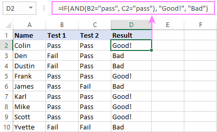
Important note! The AND function checks all the conditions, even if the already tested one(s) evaluated to FALSE. Such behavior is a bit unusual since in most of programming languages, subsequent conditions are not tested if any of the previous tests has returned FALSE.
In practice, a seemingly correct IF statement may result in an error because of this specificity. For example, the below formula would return #DIV/0! ("divide by zero" error) if cell A2 is equal to 0:
=IF(AND(A2<>0, (1/A2)>0.5),"Good", "Bad")
The avoid this, you should use a nested IF function:
=IF(A2<>0, IF((1/A2)>0.5, "Good", "Bad"), "Bad")
For more information, please see IF AND formula in Excel.
Excel IF function with multiple conditions (OR logic)
To do one thing if any condition is met, otherwise do something else, use this combination of the IF and OR functions:
The difference from the IF / AND formula discussed above is that Excel returns TRUE if any of the specified conditions is true.
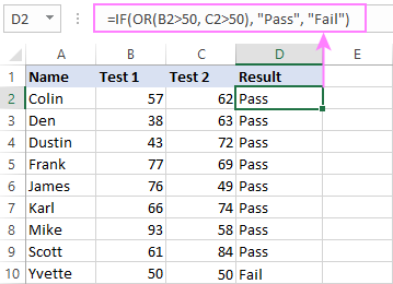
So, if in the previous formula, we use OR instead of AND:
=IF(OR(B2>50, B2>50), "Pass", "Fail")
Then anyone who has more than 50 points in either exam will get "Pass" in column D. With such conditions, our students have a better chance to pass the final exam (Yvette being particularly unlucky failing by just 1 point :)
Tip. In case you are creating a multiple IF statement with text and testing a value in one cell with the OR logic (i.e. a cell can be "this" or "that"), then you can build a more compact formula using an array constant.
For example, to mark a sale as "closed" if cell B2 is either "delivered" or "paid", the formula is:
=IF(OR(B2={"delivered", "paid"}), "Closed", "")
More formula examples can be found in Excel IF OR function.
IF with multiple AND & OR statements
If your task requires evaluating several sets of multiple conditions, you will have to utilize both AND & OR functions at a time.
In our sample table, suppose you have the following criteria for checking the exam results:
- Condition 1: exam1>50 and exam2>50
- Condition 2: exam1>40 and exam2>60
If either of the conditions is met, the final exam is deemed passed.
At first sight, the formula seems a little tricky, but in fact it is not! You just express each of the above conditions as an AND statement and nest them in the OR function (since it's not necessary to meet both conditions, either will suffice):
OR(AND(B2>50, C2>50), AND(B2>40, C2>60)
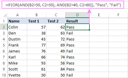
Then, use the OR function for the logical test of IF and supply the desired value_if_true and value_if_false values. As the result, you get the following IF formula with multiple AND / OR conditions:
=IF(OR(AND(B2>50, C2>50), AND(B2>40, C2>60), "Pass", "Fail")
The screenshot below indicates that we've done the formula right:
Naturally, you are not limited to using only two AND/OR functions in your IF formulas. You can use as many of them as your business logic requires, provided that:
- In Excel 2007 and higher, you have no more than 255 arguments, and the total length of the IF formula does not exceed 8,192 characters.
- In Excel 2003 and lower, there are no more than 30 arguments, and the total length of your IF formula does not exceed 1,024 characters.
Nested IF statement to check multiple logical tests
If you want to evaluate multiple logical tests within a single formula, then you can nest several functions one into another. Such functions are called nested IF functions. They prove particularly useful when you wish to return different values depending on the logical tests' results.
Here's a typical example: suppose you want to qualify the students' achievements as "Good", "Satisfactory" and "Poor" based on the following scores:
- Good: 60 or more (>=60)
- Satisfactory: between 40 and 60 (>40 and <60)
- Poor: 40 or less (<=40)
Before writing a formula, consider the order of functions you are going to nest. Excel will evaluate the logical tests in the order they appear in the formula. Once a condition evaluates to TRUE, the subsequent conditions are not tested, meaning the formula stops after the first TRUE result.
In our case, the functions are arranged from largest to smallest:
=IF(B2>=60, "Good", IF(B2>40, "Satisfactory", "Poor"))
Naturally, you can nest more functions if needed (up to 64 in modern versions).

For more information, please see How to use multiple nested IF statements in Excel.
Excel IF array formula with multiple conditions
Another way to get an Excel IF to test multiple conditions is by using an array formula.
To evaluate conditions with the AND logic, use the asterisk:
To test conditions with the OR logic, use the plus sign:
To complete an array formula correctly, press the Ctrl + Shift + Enter keys together. In Excel 365 and Excel 2021, this also works as a regular formula due to support for dynamic arrays.
For example, to get "Pass" if both B2 and C2 are greater than 50, the formula is:
=IF((B2>50) * (C2>50), "Pass", "Fail")

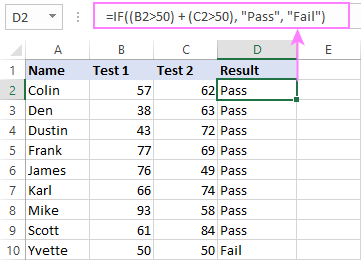
In my Excel 365, a normal formula works just fine (as you can see in the screenshots above). In Excel 2019 and lower, remember to make it an array formula by using the Ctrl + Shift + Enter shortcut.
To evaluate multiple conditions with the OR logic, the formula is:
=IF((B2>50) + (C2>50), "Pass", "Fail")
Using IF together with other functions
This section explains how to use IF in combination with other Excel functions and what benefits this gives to you.
Example 1. If #N/A error in VLOOKUP
When VLOOKUP or other lookup function cannot find something, it returns a #N/A error. To make your tables look nicer, you can return zero, blank, or specific text if #N/A. For this, use this generic formula:
For example:
If #N/A return 0:
If the lookup value in E1 is not found, the formula returns zero.
=IF(ISNA(VLOOKUP(E1, A2:B10, 2,FALSE )), 0, VLOOKUP(E1, A2:B10, 2, FALSE))
If #N/A return blank:
If the lookup value is not found, the formula returns nothing (an empty string).
=IF(ISNA(VLOOKUP(E1, A2:B10, 2,FALSE )), "", VLOOKUP(E1, A2:B10, 2, FALSE))
If #N/A return certain text:
If the lookup value is not found, the formula returns specific text.
=IF(ISNA(VLOOKUP(E1, A2:B10, 2,FALSE )), "Not found", VLOOKUP(E1, A2:B10, 2, FALSE))

For more formula examples, please see VLOOKUP with IF statement in Excel.
Example 2. IF with SUM, AVERAGE, MIN and MAX functions
To sum cell values based on certain criteria, Excel provides the SUMIF and SUMIFS functions.
In some situations, your business logic may require including the SUM function in the logical test of IF. For example, to return different text labels depending on the sum of the values in B2 and C2, the formula is:
=IF(SUM(B2:C2)>130, "Good", IF(SUM(B2:C2)>110, "Satisfactory", "Poor"))
If the sum is greater than 130, the result is "good"; if greater than 110 – "satisfactory', if 110 or lower – "poor".
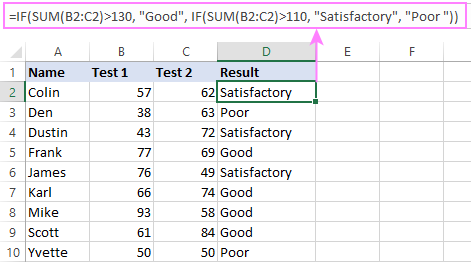
In a similar fashion, you can embed the AVERAGE function in the logical test of IF and return different labels based on the average score:
=IF(AVERAGE(B2:C2)>65, "Good", IF(AVERAGE(B2:C2)>55, "Satisfactory", "Poor"))
Assuming the total score is in column D, you can identify the highest and lowest values with the help of the MAX and MIN functions:
=IF(D2=MAX($D$2:$D$10), "Best result", "")
=IF(D2=MAX($D$2:$D$10), "Best result", "")
To have both labels in one column, nest the above functions one into another:
=IF(D2=MAX($D$2:$D$10), "Best result", IF(D2=MIN($D$2:$D$10), "Worst result", ""))

Likewise, you can use IF together with your custom functions. For example, you can combine it with GetCellColor or GetCellFontColor to return different results based on a cell color.
In addition, Excel provides a number of functions to calculate data based on conditions. For detailed formula examples, please check out the following tutorials:
Example 3. IF with ISNUMBER, ISTEXT and ISBLANK
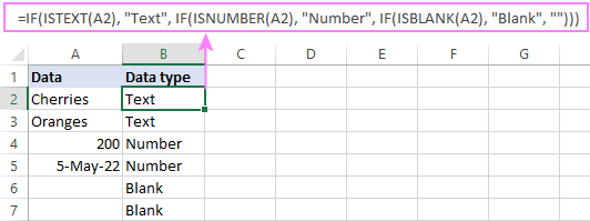
To identify text, numbers and blank cells, Microsoft Excel provides special functions such as ISTEXT, ISNUMBER and ISBLANK. By placing them in the logical tests of three nested IF statements, you can identify all different data types in one go:
=IF(ISTEXT(A2), "Text", IF(ISNUMBER(A2), "Number", IF(ISBLANK(A2), "Blank", "")))
Example 4. IF and CONCATENATE
To output the result of IF and some text into one cell, use the CONCATENATE or CONCAT (in Excel 2016 - 365) and IF functions together. For example:
=CONCATENATE("You performed ", IF(B1>100,"fantastic!", IF(B1>50, "well", "poor")))
=CONCAT("You performed ", IF(B1>100,"fantastic!", IF(B1>50, "well", "poor")))
Looking at the screenshot below, you'll hardly need any explanation of what the formula does:

IF ISERROR / ISNA formula in Excel
The modern versions of Excel have special functions to trap errors and replace them with another calculation or predefined value - IFERROR (in Excel 2007 and later) and IFNA (in Excel 2013 and later). In earlier Excel versions, you can use the IF ISERROR and IF ISNA combinations instead.
The difference is that IFERROR and ISERROR handle all possible Excel errors, including #VALUE!, #N/A, #NAME?, #REF!, #NUM!, #DIV/0!, and #NULL!. While IFNA and ISNA specialize solely in #N/A errors.
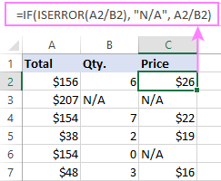
For example, to replace the "divide by zero" error (#DIV/0!) with your custom text, you can use the following formula:
=IF(ISERROR(A2/B2), "N/A", A2/B2)
And that's all I have to say about using the IF function in Excel. I thank you for reading and hope to see you on our blog next week!
Practice workbook for download
Excel IF multiple criteria - examples (.xlsx file)
 by
by
4506 comments
Hi! Need help with a formulae that returns both value and results.
Example:
Cell D4 = “Comply, ## days” or “Non Comply, ## days”
Thanks!
Hi,
I wanted to calculate number of late punch in with the criteria as follows:
If a person comes late for 6 days the 1 day leave considered, if >6 and = 9 then 1.5 days, if >9 = 12, 2 days,if >12 = 15, 2.5 days, if >15=18, 3 days and so on.
Hi everyone,
I am trying to use a formula to calculate a value using multiplication depending on different text.
Say C16 is 6 then I want to be able to get the below = values:
IF SSC then C16*390*1.1 = 2574
IF SO then C16*360 = 2160
IF SS then C16*390 = 2340
IF PSO then C16*320 = 1920
IF PSS then C16*360 = 2160
I have tried adding more criteria to the below but can't get it to work. What am I doing wrong??
=IF(D16:D18="SSC",C16*390*1.1)
Many thanks and all help is much appreciated!
Hi Melina,
You should use the nested IFs and absolute cell references with the $ sign in your formula. It will look like this:
=IF($D$16:$D$20="SSC", $C$16*390*1.1, IF($D$16:$D$20="SO", $C$16*360, IF($D$16:$D$20="SS", $C$16*390, IF($D$16:$D$20="PSO", $C$16*320, IF($D$16:$D$20="PSS", $C$16*360, "")))))
Where $C$16 is the cell that contains your number 6, $D$16:$D$20 is the range with the text values.
Dear Sir/Madam,
Thank you so much. I just learned something new. I have only one question to ask relating to one of my project.
How will I use the nested if condition(or other if-conditions) to get the difference of two cells. And the difference must always rounded down to the decimal points provided below.
a) 0.00
b) 0.25
c) 0.50
d) 0.75
e) 1.00
Example:
1) If my difference is 7.15 then my rounded value will be 7.00
2) If my difference is 7.48 then my rounded value will be 7.25
3) If my difference is 7.74 then my rounded value will be 7.50
4) If my difference is 7.99 then my rounded value will be 7.75
Please I really need your help on this problem.
Thank you again.
Aloysius Agobe
Dear Aloysius,
If I understand your task right, you don't actually need to use the IF function. Please try to enter the following formula in cell C1 to get the result you need:
=FLOOR((A1-B1),0.25)
Where A1 and B1 are two cells with the numeric values from which you are trying to find the difference.
Hope this will help.
Hi again,
If my column as a different text value can I do a count for each of the values in the same column..I need to know how many "Retiree Family", "Active Individual" etc.. not sure if this can be done in a formula or not.
Thanks for your help...
Maria,
If I understand your task correctly, the COUNTIF function will work for you, e.g.:
=COUNTIF(A1:A13,"Retiree Family")
You can find more information about COUNTIF in this article on our blog.
Hope this will help.
Hi
How many If(and formula can be nested in windows 10? I did 8 and am getting too many nesting for this formula. Am I doing something wrong?
=IF(AND(B198="G01",E198=4,I198="E"),"Retiree Family",IF(AND(B198="G01",E198=1,I198="E"),"Retiree Individual",IF(AND(B198="M04",E198=4,I198="E"),"Active Family",IF(AND(B198="M04",E198=1,I198="E"),"Active Individual",IF(AND(B198="G04",E198=1,I198="E"),"G04 Retiree Individual",IF(AND(B198="G04",E198=4,I198="E"),"G04 Retiree Family",IF(AND(B198="G03",E198=4,I198="E"),"G03 Retiree Family",IF(AND(B198="G03",E198=4,I198="E"),"G03 Retiree Individual"0)))))))
Hi Maria,
Please note that in Excel 2016 – 2007 you can nest up to 64 IF functions in one formula. In Excel 2003 and lower, up to 7 nested IF functions can be used.
At first view your formula is missing a comma before 0 and one closing parenthesis at the end. Please correct the formula and check if it works.
If it doesn't, then describe your task in more detail and send us a small sample workbook with your source data and the result you want to get to support@ablebits.com.
Please shorten your table to 10-20 rows / columns and don't forget to include the link to your comment in the email.
We'll look into the issue and try to help.
Hi, hope all of you are having a great time i am looking to do a formula but can do it, need some assistance
IF range from 31% to 32.99% nee to show $0.20
some body can help me with it please?
hey can anyone figure this out.....I need a formula that will grab just a specific item with 3 conditions. I have a column with part name, Vendor, and number of each item they are proving us. so I want a formula that will grab individual item a specific vendor is providing us and the amount they providing.
Can you please help me when I have problem with this formula
I have tried:
=if cell U4 Empty Result on cell X4 waiting if Cell U4 paid Result on cell X4 Hold ifCell U4 Date Result on cell X4 Work Don
=IF(U4,"Agency","Waiting")=if(U4,Paid,"Hold"))
I have one:
If cell on spreadsheet "B" contains a value that is = to a cell on spreadsheet "A", then if true=paid, false="-".
how would that formula be written?
I have tried:
=if('Transaction Register'!I:I=G13,"PAID","-")
this to me says that if a cell in 'transaction register'!I:I=the cell on current sheet, then paid if true, and - if false
thanks.
Hi. I need help on this.
I have 2 separate tabs of spreadsheet. Spreadsheet A - main list, Spreadsheet B - price list. I need to populate the price from Spreadsheet B into Spreadsheet A, but on conditions that only the column A and column B (eg. Supplier, Item) in Spreadsheet B must match column A and column B in Spreadsheet A before it can populate into Spreadsheet A. How can I use the If/And formula to achieve this?
I tried this, but it doesn't work:
=if((And(A2=(vlookup(A2,sosupplier,2,false)),B2=(vlookup(B2,soprice,2,false)),(vlookup(B2,soprice,7,false)),"no")))
Can you please help me when I have problem like this.
IF A =1, B=2 C=3....I=9
If I have AB in A1 cell I want answer in B1 like "12" if I have ABD in A2 cell then I want answer in B2 like "124"
Please help.
thanks
Tejas
I need to make the value in column J be dependent on one of 3 variables found in column D. Example: column J is 45 if column D is “X” column J is 40 if column D is “Y” and so on. I’ve been trying for 12 hours and am very frustrated, can anyone help me please?
I'm using a matrix to represent a recruiting schedule with 1 or 0. When a recruit joins (satisfies the condition of 1), then they receive a fixed funding amount that year and the subsequent 4 years. More simply, if a recruit joins in 2018, they receive fixed funding in 2018 through 2022. How can I write an if/then statement that returns the funding value to the cell in which the if/then statement is written and the next 4 cells in the row?
I am trying to create a formula that will return either "Unable" or "Able" based on the three criteria below. these three are the combination of options for the three cells that should come back as "Unable"
1. L2=yes, M2=no, N2=yes
2. l2=no,m2=yes,n2=yes
3. l2=no,m2=no,n2=yes
This is the formula i have, but it is not working. can anyone help?
=if(OR(AND(L2=yes, M2=no, N2=yes), AND(l2=no, m2=yes, n2=yes), AND(l2=no, m2=no, n2=yes)),”Unable”,”Able”)
i am looking to have a return of "unable" if any one of these three criteria are met.
thanks
Hello,
Please note that text values are always enclosed in "double quotes" in Excel formulas. So the correct formula should be as follows:
=IF(OR(AND(L2="yes",M2="no",N2="yes"),AND(L2="no",M2="yes",N2="yes"),AND(L2="no",M2="no",N2="yes")),"Unable","Able")
Hope this is what you need.
Hi,
yes, thank you so much! I should have realized that.
How would the equation change if I wanted to add to it that if any of the areas are left blank, it should also have a return of "unable"
I could add in the various =AND equations, but that would be a huge list of them. is there another way to do this?
Hi,
If you want to return "Unable" when any of cells L2:N2 is empty, then just add one more condition to the formula. It will look like this:
=IF(OR(AND(L2="yes",M2="no",N2="yes"),AND(L2="no",M2="yes",N2="yes"),AND(L2="no",M2="no",N2="yes"),OR(ISBLANK(L2),ISBLANK(M2),ISBLANK(N2))),"Unable","Able")
Hopefully it will help you.
Can anyone help me with this?
I want to make a formula for cell B12 (as example) that says
if A1=1 AND A2=1 make the value 100
if A1=1 AND A2=2 make the value 150
if A1=1 AND A2=3 make the value 200
if A1=2 AND A2=1 make the value 250
if A1=2 AND A2=2 make the value 300
if A1=2 AND A2=3 make the value 350
if A1=3 AND A2=1 make the value 400
if A1=3 AND A2=2 make the value 450
if A1=3 AND A2=3 make the value 500
How do I make this into one formula?
Hi All,
can somebody please help with the following?
I am trying to do 3 conditions, using nested "IF" with "AND" functions and "IF" with "OR" functions. Let's assume cell c3=2 and cell c4=3. what I am trying to achieve is the following, if c3=2 and c4=3 than display 100, if c32 or c43 then display 50, if c32 and c43 then display 0.
I have tried the following formula which covers the first two conditions, but I cannot figure out how to get the third condition working. TIA
=IF(AND(C3=2,C4=3),"100",IF(OR(C32,C43),"50","0"))
=IF(AND(C3=2,C4=3),"100",IF(OR(C32,C43),"50",IF(AND(C3"2",C4"3"),"0")))
I want mark on the basis of the cell value. If Cell contained Y gives 1 mark and N contain 0. How can i use the IF(and) or if(or) function
Hello, Nirav,
Please see the examples of the IF and OR/AND functions usage in the first part of this article.
If none of the described cases work for you, then please provide us with more details regarding your task. You can send us a small table with sample data and the result you want to get to support@ablebits.com. Please don't forget to include the link to your blog comment into an email.
We'll look into your task and try to help.
Wage rate 201 Rupes
1000 wages to 6 %
1001 to 2000 wages 4%
2001 to above 2.5% commotion
A1 Passed C1 Passed E1 Passed G1Failed I1Failed. I Want J1 to be if 3/5 Cells are "Passed". Final Result is Passed, if not Failed.
Hello,
Please try the following formula:
=IF((COUNTIF(A1,"Passed")+COUNTIF(C1,"Passed")+COUNTIF(E1,"Passed")+COUNTIF(G1,"Passed")+COUNTIF(I1,"Passed"))>=3,"Passed","Failed")
Hope it will help you.
Hi,
How to link together those two formulas to be able create formula with multiply conditions:
=IF(I9=N7;O9*N9;O9*M9)
Thanks in advance!
Hi,
How to link together those two formulas to be able create formula with multiply conditions:
=IF(I9=N7;O9*N9;O9*M9)
Thanks in advance!
hi everyone I have an issue with the formula : I need to transfer a project ID if column x has a value between 3 and 5 mln and column Y =yes I cannot make it work with a nested IF any suggestions - what am I doing wrong?
I perform monthly commissions for my company. We have different calculations depending on the goal that's met.
For example:
2% Goal 1: $50
4% Goal 2: $100
Scenario 1 goal 1 met:
Attainment: $75
Commission is calculated by ($75-$50)*2% = commission 1
Did not meet goal 2
Scenario 2 both goals met:
Attainment: $125
Rep is eligible for 2 payouts.
($100-$50)*2%= commission 1
($125-$100)*4%=commission 2
What I am trying to create is a formula that will determine if the criteria is met and to use the appropriate calculation. Can anyone help me with this?
I want to put a formula if
Gross salary is below than Rs.7500 then Professional Tax should 0,
if greater than 7500 and less than 10000 then PT should 175 and
if gross salary is greater than 10000 then PT should 200
How to write it? please guide
Hi Try this below example with your scenario;
Formula - =IF(B1<7500,"0",IF(B110000,"200","")))
Name Salary PT
A 19,131 200
B 11,937 200
C 7,984 175
D 18,692 200
E 13,105 200
F 17,416 200
G 7,238 0
Appreciate it if anyone could assist:
How would I create this in an excel cell:
if object is between $1-$2500, the cost would be $10 for the first $500 plus $4 for each additional $10 or a fraction thereof, to and including $2500.
Thank you.
Hi Svetlana,
I am trying to find a formula to resolve the following:
Column A has three criteria and column B has five criteria. I would like to have the summed value in column C for each criteria in column A that satisfies one or more of the criteria in column B, and return the value if it is >0.
Thanks.
An Ambulance Move form Their Stand Under Following Levels
01 E Level Response Time is 12 Min "Not Delayed" else "Delayed"
02 D Level Response Time is 12 Min "Not Delayed" else "Delayed"
03 C Level Response Time is 15 Min "Not Delayed" else "Delayed"
04 B Level Response Time is 15 Min "Not Delayed" else "Delayed"
05 A Level Response Time is 30 Min "Not Delayed" else "Delayed"
06 O Level Response Time is 30 Min "Not Delayed" else "Delayed"
Kindly Solve My Problem in Any Condition Plz
I need to provide the following reference:
If(H14-(F17-G17)>=4000,4000)
We have a 4000 gallon storage tank, I need to track the amount of available product between loads but cannot exceed 4000 gallons.
Dear,
can anybody help for below table with Vlookup. i need to take actual values f column A
A B C
SO-AZM-043847 Danat Al Emarat Hospita l- (AUH) 213484
SO-AZM-043847 Danat Al Emarat Hospita l- (AUH) 213485
SO-AZM-043847 Danat Al Emarat Hospita l- (AUH) 213486
A B C
SO-AZM-043847 Danat Al Emarat Hospita l- (AUH) ?
SO-AZM-043847 Danat Al Emarat Hospita l- (AUH) ?
SO-AZM-043847 Danat Al Emarat Hospita l- (AUH) ?
Please help. I am trying (and failing) to put a medical score on excel. Each of the parameters has a cell#. These all have points value.
POINTS:
parameters 1 2 3
___________ _____ ________ _______
Bilirubin 3
Albumin >3.5 2.8-3.5 <2.8
INR 2.3
or PT 6
Ascites none (1) mild-mod (2 or 3) severe (4)
Encephalopathy none (1) mild-mod (2 or 3) severe (4)
total of 5 criteria are used in this calculation, but INR and PT can be used interchangeably.
Class A: score =10
so if Bilirubin is 3.5, Albumin is 2, INR is 2, Ascite and Encephalopathy are both severe, would yield a score 14. That would be a class C.
so want to write a formula that would sum up these possibilities and yield a class.
Please help.
Thank you very very much in advance.
Hi I need help for a formula for the following
cell D4 = value of C5 if cell D2 contains 1
thank you
Hello,
If I understand your task correctly, please try the following formula:
=IF(D2=1,C5,"")
Hope it will help you.
Hello I need an if and statement that sums. If column M has "active" or "inactive" then sum it and and put it in column Z. Then I need the same if column M has (Potential or No sale) put in column AA. Thank You
Hello,
For me to understand the problem better, please send me a small sample workbook with your source data and the result you expect to get to support@ablebits.com. Please don't worry if you have confidential information there, we never disclose the data we get from our customers and delete it as soon as the problem is resolved.
Please also don't forget to include the link to this comment into your email.
I'll look into your task and try to help.
Ps could u help...if I type something in A1, I want to show Name code automatically in A2.
If A1 is Anil, then i want A2 to show 9
If A1 is Sunil, then i want A2 to show 10
If A1 is Peter, then i want A2 to show 11
If A1 is Harry, then i want A2 to show 12
Ps help me
Thanks!!
Hello, Anil,
If I understand your task correctly, please try to enter the following formula in cell A2:
=IFS(A1="Anil",9,A1="Sunil",10,A1="Peter",11,A1="Harry",12)
Hope this is what you need.
Hi,
Can anyone help me to create this formula,
If the total value is equals to:
1. 0 - 2,000, then times it by 0.071
2. 2,001 - 25,000, times it by 0.075
3. 25,001 - 75,000, times it by 0.085
And so on... can anyone help me with the correct formula please!
Thank you!
Hello,
If I understand your task correctly, please try the following formula:
=IFS(A1<=2000,A1*0.071,A1<=25000,A1*0.075,A1<=75000,A1*0.085)
Hope it will help you.
DEAR SIR/MADAM
MY BILL NO. IS HIC/01..CAN I SERIAL WISE HIC/02,03,04..PLZ GIVE ME A FORMULA
Hi,
Can u help me to build a Formula. If A2 Contains "ce",and v2q2,0,v2)
I am trying to do an if and or using this scenario written out and am not sure how to do it: if cell K3 is zero, then just use L3 in M3, and if cell K3 is populated (not zero), still use L3 in M3 (no aggregation), however if K3 is populated but L3 is not, use the value of K3 in M3. Any ideas?
Hello,
For me to understand the problem better, please send me a small sample workbook with your source data and the result you expect to get to support@ablebits.com. Please don't worry if you have confidential information there, we never disclose the data we get from our customers and delete it as soon as the problem is resolved.
Please also don't forget to include the link to this comment into your email.
I'll look into your task and try to help.
Hello Svetlana,
pls. provide formula for this :
If C1= start with “ST” and D1=”18” then result “214810”
If C1= start with “S0” and D1=”18” then result “214810”
If C1= start with “S0” and D1=”9” then result “214800”
If C1= start with “EX” and D1=” ” then result “ ”
If C1= start with “ST” and D1=”9” then result “CHECK”
Thanks in advance
Hello,
If I understand your task correctly, please try the following formula:
=IF(AND(LEFT(C1,2)="ST",D1=18),"214810",IF(AND(LEFT(C1,2)="S0",D1=18),"214810",IF(AND(LEFT(C1,2)="S0",D1=9),"214800",IF(AND(LEFT(C1,2)="EX",D1=""),"",IF(AND(LEFT(C1,2)="ST",D1=9),"CHECK","")))))
Hope this will help.
Thank you very much
Hi there,
I am having issues with my If(And formula. Here's the formula =IF(AND(AQ2=AR2=AS2),"No Change",IF(AND(AR2=AS2,AQ2AR2,AQ2AS2),"Title Change Only",IF(AND(AQ2=AS2,AR2AS2,AR2AQ2),"Job Code Change",IF(AND(AQ2=AR2,AS2AR2,AS2AQ2),"Comp Change",IF(AND(AQ2AR2,AQ2AS2),"Comp & Code Change","ERROR")))))
Where columns AQ, AR and AS are:
AQ= Yes or No, AR= YES or NO, AS=YES or no
Hello,
If I understand your task correctly, please try the following formula:
=IF(AND(AQ2=AR2,AQ2=AS2),"No Change",IF(AND(AR2=AS2,AQ2<>AR2,AQ2<>AS2),"Title Change Only",IF(AND(AQ2=AS2,AR2<>AS2,AR2<>AQ2),"Job Code Change",IF(AND(AQ2=AR2,AS2<>AR2,AS2<>AQ2),"Comp Change",IF(AND(AQ2<>AR2,AQ2<>AS2),"Comp & Code Change","ERROR")))))
Hope this will help you with your task.
I need the similar formula but want to select the value from my excel cell.
Please share the formula
Thanks in Advance
Hi Sakib,
Instead of typing a value directly in a formula, enter a reference to the cell containing the value.
Thanks a lot Dear ... its working :)
hi,
i am trying to create reference to a cell in IF function.
e.g. IF(k19<0, "f18=k19","0") instead of applying f18=k19 its showing result as f18=k19 as text. i changed the cell format etc. but .....
Hello MAQBOLL, when you use "" you are telling to excel to write as a text whatever is between "" For example "f18=k19" will be written in your cell f18=f19 just like that.
If you want that F18 be equal to K19 if K19=0 then...
Try writing this formula directly in F18 cell
=IF(K19<0,K19,0)
Hope this helps
Hello Svetlana,
pls. help on this :
If C1= start with “ST” and D1=”18” then result “214810”
If C1= start with “S0” and D1=”18” then result “214810”
If C1= start with “S0” and D1=”9” then result “214800”
If C1= start with “EX” and D1=” ” then result “ ”
If C1= start with “ST” and D1=”9” then result “CHECK”
Try this in the cells in column c
@IF(AND(A1="Complex",B1=6),"Exceeded","")
can someone help me in creating a formula in excel using nested IFs?
basically, what I need is:
IF column A is equal to "Complex" and value of column B is 6 the column C would indicate "Exceeded"
IF column A is equal to "Non Complex" and value of column B is 4 the column C would indicate "Exceeded"
Thanks in advance!
basically, what I need is:
IF column A is equal to "Complex" and value of column B is 6 the column C would indicate "Exceeded"
Hello,
If I understand your task correctly, please try the following formula:
=IF(AND(A1="Complex",B1=6),"Exceeded",IF(AND(A1="Non Complex",B1=4),"Exceeded",""))
Hope it will help you.
name. total result position
robi. 354. pass. 2nd
moni. 456. pass. 1st
kobi. 123. fail. Na
tuni. 212. fail. Na.
What is the formula to evaluate position whose result passed.
Hi, I just cannot get this to work.. I'm making an invoice template. And I want an IBAN number to appear only if I select English from the dropdown menu. And it has to be one relative to a bank account I choose from another.
something like:
if A1="eng" and B1="bank1" = IBAN1,
if A1="eng" and B1="bank2" = IBAN2,
if A1="cz" = ""
nevermind, I figured it out.
=IF((AND(D1="eng", B11="bank1")), IBAN1, IF( (AND(D1="eng", B11="bank2")), "IBAN2", "" ))
How to write formula in R colunm using or condition
if q>=2 (1 days deduction)
if q>=40 (2 days decuction)
if q>=6 (3 days decuction)
if q>=8 (4 days decuction)
if q>=10 (5 days decuction)
if q>=12 (6 days decuction)
if q>=14 (7 days decuction)
if q>=16 (8 days decuction)
Hello,
For me to understand the problem better, please send me a small sample workbook with your source data and the result you expect to get to support@ablebits.com. Please don't worry if you have confidential information there, we never disclose the data we get from our customers and delete it as soon as the problem is resolved.
Please also don't forget to include the link to this comment into your email.
I'll look into your task and try to help.
TRY THIS
=IF(Q>=2,(NO OF DAYS) -1)
can anyone help with this formula, looking at two fields:
Due date e.g. 01/01/18 = Cell S2
Paid = True/ False = Cell Q2
Formula
If paid = "Paid"
if >today & false = "Not due"
if <today & false = "Overdue"
Thanks
Hello,
Please try the following formula:
=IF(Q2,"Paid",IF(S2>=TODAY(),"Not due","Overdue"))
Hope it will help you.
I want to use 3 conditions in once cell using If, as below sample.
The condition is =I(E9>0.79,"PASSED","FAILED"). On that condition, if I'm going to drag down the cell it will show nothing or blank, but its not appearing blank, its showing the "PASSED or FAILED".
Score Date Remarks
80% 23-Nov-17 PASSED
Hello, Wyndel,
As far as I can see from your formula, it contains only one condition (E9>0.79). Please specify what two other conditions are and what should be displayed as the result.
I’ll try to adjust your formula for your needs.