The tutorial shows how to compare text strings in Excel for case-insensitive and exact match. You will learn a number of formulas to compare two cells by their values, string length, or the number of occurrences of a specific character, as well as how to compare multiple cells.
When using Excel for data analysis, accuracy is the most vital concern. Incorrect information leads to missed deadlines, misjudged trends, wrong decisions and lost revenues.
While Excel formulas are always perfectly true, their results may be wrong because some flawed data penetrated into the system. In this case, the only remedy is to check data for accuracy. It's no big deal to compare two cells manually, but it's next to impossible to spot the differences between hundreds and thousands of text strings.
This tutorial will teach you how to automate the tedious and error-prone task of cell comparison and what formulas are best to use in each particular case.
How to compare two cells in Excel
There are two different ways to compare strings in Excel depending on whether you seek case-sensitive or case-insensitive comparison.
Case-insensitive formula to compare 2 cells
To compare two cells in Excel ignoring case, use a simple formula like this:
=A1=B1
Where A1 and B1 are the cells you are comparing. The result of the formula are Boolean values TRUE and FALSE.
If you want to output your own texts for matches and differences, embed the above statement in the logical test of the IF function. For example:
=IF(A1=B1, "Equal", "Not equal")
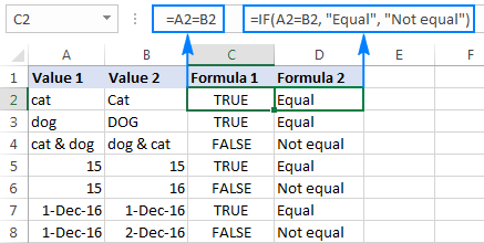
As you see in the screenshot below, both formulas compare text strings, dates and numbers equally well:
Case-sensitive formula to compare strings in Excel
In some situations, it may be important not only to compare text values of two cells, but also to compare the character case. Case-sensitive text comparison can be done using the Excel EXACT function:
Where text1 and text2 are the two cells you are comparing.
Assuming your strings are in cells A2 and B2, the formula goes as follows:
=EXACT(A2, B2)
As the result, you get TRUE for text strings match exactly including the case of each character, FALSE otherwise.
If you want the EXACT function to deliver some other results, embed it in an IF formula and type your own text for value_if_true and value_if_false arguments:
=IF(EXACT(A2 ,B2), "Exactly equal", "Not equal")
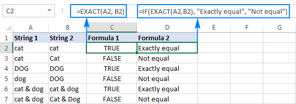
The following screenshot shows the results of the case-sensitive string comparison in Excel:
How to compare multiple cells in Excel
To compare more than 2 cells in a row, use the formulas discussed in the above examples in combination with the AND operator. The full details follow below.
Case-insensitive formula to compare more than 2 cells
Depending on how you want to display the results, utilize one of the following formulas:
=AND(A2=B2, A2=C2)
or
=IF(AND(A2=B2, A2=C2), "Equal", "Not equal")
The AND formula returns TRUE if all of the cells contain the same value, FALSE if any value is different. The IF formula outputs the labels that you type in it, "Equal" and "Not equal" in this example.
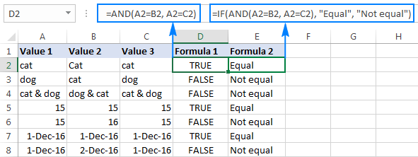
As demonstrated in the screenshot below, the formula works perfectly with any data types - text, dates and numeric values:
Case-sensitive formula to compare text in several cells
To compare multiple strings to each other to see if they match exactly, use the following formulas:
=AND(EXACT(A2,B2), EXACT(A2, C2))
Or
=IF(AND(EXACT(A2,B2), EXACT(A2, C2)),"Exactly equal", "Not equal")
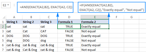
Like in the previous example, the first formula delivers TRUE and FALSE values, whereas the second one displays your own texts for matches and differences:
Compare a range of cells to a sample cell
The following examples show how you can verify that all cells in a given range contain the same text as in a sample cell.
Case-insensitive formula to compare cells to a sample text
If the character case does not really matter, you can use the following formula to compare cells to a sample:
In the logical test of the IF function, you compare two numbers:
- The total number of cells in a specified range (the number of rows multiplied by the number of columns), and
- The number of cells containing the same value as in the sample cell (returned by the COUNTIF function).
Assuming the sample text is in C2 and the strings to compare are in the range A2:B6, the formula goes as follows:
=ROWS(A2:B6)*COLUMNS(A2:B6)=COUNTIF(A2:B6,C2)
To make the results more user-friendly, i.e. output something like "All match" and "Not all match" instead of TRUE and FALSE, use the IF function like we did in the previous examples:
=IF(ROWS(A2:B6)*COLUMNS(A2:B6)=COUNTIF(A2:B6,C2),"All match", "Not all match")
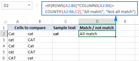
As shown the above screenshot, the formula perfectly copes with a range of text strings, but it can also be used to compare numbers and dates.
Case-sensitive formula to compare strings to a sample text
If the character case makes a difference, you can compare strings to the sample text using the following array formulas.
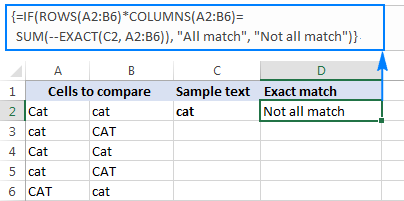
With the source range residing in A2:B6 and the sample text in C2, the formula takes the following shape:
=IF(ROWS(A2:B6)*COLUMNS(A2:B6)=SUM(--EXACT(C2, A2:B6)), "All match", "Not all match")
Unlike regular Excel formulas, array formulas are completed by pressing Ctrl + Shift + Enter. If entered correctly, Excel encloses the array formula in {curly braces}, as shown in the screenshot:
To identify if a certain value is present or absent in a range, please see Check if a value exists in a range.
How to compare two cells by string length
Sometimes you may want to check if the text strings in each row contain an equal number of characters. The formula for this task is very simple. First, you get the string length of two cells using the LEN function, and then compare the numbers.
Supposing the strings to be compared are in cells A2 and B2, use either of the following formulas:
=LEN(A2)=LEN(B2)
Or
=IF(LEN(A2)=LEN(B2), "Equal", "Not equal")
As you already know, the first formula returns Boolean values TRUE or FALSE, whereas the second formula outputs your own results:
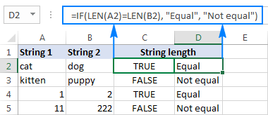
As demonstrated in the screenshot above, the formulas work for text strings as well as numbers.
Tip. If two seemingly equal strings return different lengths, most likely the problem is in leading or trailing spaces in one or both cells. In this case, remove extra spaces using the TRIM function. The detailed explanation and formula examples can be found here: How to trim spaces in Excel.
Compare two cells by occurrences of a specific character
This is the last example in our Excel Compare Strings tutorial, and it shows a solution for a rather specific task. Supposing, you have 2 columns of text strings that contain a character important to you. Your goal is to check whether two cells in each row contain the same number of occurrences of a given character.
To make things clearer, consider the following example. Let's say, you have two lists of orders shipped (column B) and received (column C). Each row contains orders for a specific item, whose unique identifier is included in all order IDs and is listed in the same row in column A (please see the screenshot below). You want to make sure that each row contains an equal number of shipped and received items with that specific ID.
To solve this problem, write a formula with the following logic.
- Firstly, replace the unique identifier with nothing using the SUBSTITUTE function:
SUBSTITUTE(A1, character_to_count,"") - Then, calculate how many times the unique identifier appears in each cell. For this, get the string length without the unique identifier and subtract it from the total length of the string. This part shall be written for cell 1 and cell 2 individually, for example:
LEN(cell 1) - LEN(SUBSTITUTE(cell 1, character_to_count, ""))
and
LEN(cell 2) - LEN(SUBSTITUTE(cell 2, character_to_count, "")) - Lastly, you compare these 2 numbers by placing the equality sign (=) in between the above parts.
LEN(cell 2) - LEN(SUBSTITUTE(cell 2, character_to_count, ""))
In our example, the unique identifier is in A2, and the strings to compare are in cells B2 and C2. So, the complete formula is as follows:
=LEN(B2)-LEN(SUBSTITUTE(B2,$A2,""))=LEN(C2)-LEN(SUBSTITUTE(C2,$A2,""))
The formula returns TRUE if cells B2 and C2 contain an equal number of occurrences of the character in A2, FALSE otherwise. To make the results more meaningful for your users, you can embed the formula in the IF function:
=IF(LEN(B2)-LEN(SUBSTITUTE(B2, $A2,""))=LEN(C2)-LEN(SUBSTITUTE(C2, $A2,"")), "Equal", "Not equal")
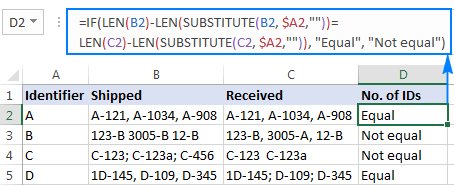
As you can see in the screenshot above, the formula works perfectly despite a couple of additional complications:
- The character to be counted (unique identifier) can appear anywhere in a text string.
- The strings contain a variable number of characters and different separators such as semicolon, comma or space.
This is how you compare strings in Excel. To have a closer look at the formulas discussed in this tutorial, you are welcome to download our sample sheet below. I thank you for reading and hope to see you on our blog next week!
Practice workbook for download
Excel - compare strings examples (.xlsx file)
 by
by
61 comments
Hello, thanks for all your helpful answers. I there a way to identify the presence of a word or phrase that appears within other text in one column and enter a flag (eg, "X") in another column.
I have a list of names that includes gender and other information and I want additional columns that identifies the gender.
Appreciate any comments!
Hi! The following tutorial should help: How to find substring in Excel. I hope it’ll be helpful. If something is still unclear, please feel free to ask.
Hello,
I want to compare multiple columns, such that if they have the same text, it returns "no". If one cell text is different from the rest, it should return that cell that is different from the rest. Thanks.
Hi! Without seeing your source data and desired result, it is difficult to recommend a formula to you. Perhaps this article will be helpful to you: How to compare two columns in Excel for matches and differences.
Thanks for the response.
Let's say four columns have texts 'no', 'no', 'yes', 'no'
We want to return the cell that is different from the rest, which is 'yes'.
I hope this helps.
Hi! If your data is written in 4 columns, use the TRANSPOSE function to turn the columns into rows. Use the UNIQUE function to get the list of unique values in these cells. Use the COUNTIF function to count how many times each value is written. Then use INDEX MATCH function to specify the value that is written the smallest number of times.
If I understand your task correctly, the following formula should work for you:
=INDEX(UNIQUE(TRANSPOSE(A2:D2)), MATCH(MIN(COUNTIF(A2:D2,UNIQUE(TRANSPOSE(A2:D2)))), COUNTIF(A2:D2,UNIQUE(TRANSPOSE(A2:D2))),0))
Hello!
I am trying to use excel to compare a cell containing a string of 4 characters with a column of similar 4-character strings. I’m looking for 4 matches, then 3 matches, then 2, etc.
The output should be the value in the cell or cells that match the criteria.
Can someone help?
Hi! In the additional column, write this formula and copy down the column. You will get the number of matches. Then you can apply an Excel filter or the FILTER function.
=SUM(--ISNUMBER(SEARCH(MID($A$2,{1,2,3,4},1),B2)))
For more information, please read: How to find substring in Excel
Hello. Thank you very much for your tutorial.
Could I compare two pairs of cells in excel? This is, cells A and B being a pair, and cells C and D being another pair. I need to compare two pairs of cells regardless of order.
As example:
Cell A: blue - Cell B: brown / Cell C: brown - Cell D: blue
How can I compare cells A-B with cells C-D regardless of order? This is, to consider blue-brown the same as brown-blue.
Thank you very much for your help.
Eduardo
Hi!
If I understand your task correctly, the following formula should work for you:
=OR(A1&B1=C1&D1,A1&B1=D1&C1)
Hello, Alexander. Thank you very much! Yes; it solves my problem.
Your project is excellent.
Best wishes.
Eduardo
Hello again.
Following my previous question: If I need to compare not pairs but groups of 5 elements (compare two groups of 5 cells in the same row) regardless of the order of the elements in each one, Is there any alternative formula? (This because in the case of the formula you suggested me I would need to include in the formula the 120 permutations of the 5 cells).
Thank you.
Eduardo
Hi! Try using the COUNTIF function. Each value must be found 1 time.
=AND(COUNTIF(B1:B5,A1:A5)=1)
Thank you for your time and your kindness, Alexander.
I tried with the formula you suggest and it works if I put the elements in two columns. But the formula does not work if the elements are all in the same row (in different columns).
My situation is that I have near 3500 rows, and in each row I have 5 elements (in 5 columns) corresponding to one person and other 5 elements (in 5 columns) corresponding to a second person; and I need compare between the two persons (in the same row). An example:
Person 1 / Person 2
banded - striped - red - blue - green / striped - banded - red - green - blue
I need that excel says that the elements in Person 1 are the same that the elements in Person 2, regardless of they are in different order. Your formula does not work in this way. (This is for a non profit investigation regarding patterns and colors of snakes).
If you have in mind another option to do this comparison of 5 elements vs 5 elements all in the same row, and regardless of the order, I will be very grateful with you. If not, at least I can work the other cases I have (with your first formula): 2 elements vs 2 elements and 3 elements vs 3 elements (because in these cases the number of permutations is not huge).
Thank you very much, Alexander.
Eduardo
Hi! The COUNTIF function can calculate values in columns. If I understand the question correctly, try this formula:
=AND(COUNTIF(A1:E1,G1:K1)=1)
Hope this is what you need.
Very helpful and clear article.
Could you please help me with a formula that compares two cell strings (alpha numeric) and highlights the miss matched character in one of the cells.
For example:
In the first cell the string is ABC123 and in the second cell the string is ADC123
The formula should put the second string (ADC123) in a new cell, with the second character (D) highlighted.
Thank you!
Hi!
The problem cannot be solved with a single formula. Using the MID function, you can write each character in a separate column cell, and then compare these columns, as described in this tutorial: Compare two columns for matches and differences.
In addition, no Excel formula can highlight a single character in a cell by formatting.
So in my earlier query,
Cell B1 should return value 1234 since its merge A1 & A2 that has 2 digits overlapping
Cell C1 should return value 1235 since its merge A1 & A4 that has 2 digits overlapping
Cell B2 should return value 1234 since its merge A1 & A2 that has 2 digits overlapping
Cell B3 should return NIL value since A3 has no overlapping value
Cell B4 should return value 1253 since its merge A1 & A4 that has 2 digits overlapping
Cell A1 = 123
Cell A2 = 234
Cell A3 = 456
Cell A4 = 125
Thanks for all input
Hi!
I'm really sorry, looks like this is not possible with the standard Excel options.
Cell A1 = 123
Cell A2 = 234
Cell A3 = 456
Cell A4 = 125
In the above reference, when any cell in the range A1A4, has 2 digits overlapping between them, I need them to return a merged value.
How can this be done. Can someone please guide/share input pls
Regards
JS
Hello, I am struggling to get a formula to work for what I need can you please help?
I have three title columns (A)(B)(C) which represent questions that can be answered with (Y/y) or (N/n). In column (D) I would like to have the status show "No Update" or "Update" depending on the answers in each row. In order to receive and "No Update" status the responses in (A)(B)(C) must all be (Y/y), if there is a (N/n) response the status will be "Update". I also want Column D to only show "No Update"/"Update" if there is a response in columns (ABC)- if on column is blank but the other two columns have an answer column D should reflect "Update" however if all columns are blank the response should leave column D blank.
I have two working formulas that kind of work but each have a problem feature.
=IFS(A1:C1="","",A1:C1="n","Update",A1:C1="y","No Update")
will give me the right function but displays answers for each column instead of 1 response to all columns
=IF(AND(A10:C10="y"),"No Update","Update")
Gives me the correct responses in one column as needed but does not leave column D blank when unfilled columns ABC are empty.
PLEASE help I can not figure this out!!
Hello!
If I understand your problem correctly, you can use a nested IF function. The CONCAT function will help check if all three cells are empty.
=IF(AND(A10:C10="y"),"No Update",IF(CONCAT(A10:C10)="","","Update"))
This should solve your task.
What will be the formula if I want to say that "cat & dog" is the same as "dog & cat"?
Hi,
I have query which is explained in example.
Cell A2 has a sentence "MO piercing". In cell B2, i want to compare if A2 has any of the keyword like earring, anklet, piercing, jewelry. If keyword is found in A2,then B2 should show True else false.
Please help me with the query.
Hello!
To search for a string in text, use the SEARCH function. Try this formula:
=IF(SUM(--ISNUMBER(SEARCH(D1:D4,A1))),TRUE,FALSE)
D1:D4 - these are the words you are looking for (earring, anklet, piercing, jewelry). One word per cell.
I have 2 columns with percentages, Column B is % Hispanic males; Column A is % Hispanic females. (The 2 columns do NOT sum to 100% since they are percentage of whole group, not percentage within Hispanic group.)
I want to highlight both cell values in Blue if % Hispanic males equal to or more than 5 % points larger than % Hispanic females and Green if % Hispanic males is 5 % points equal to or less than % Hispanic females. (Basically, looking to highlight cells where there is the most difference and leave cells alone when the percentages are close.)
HFemale HMale
13.4% 12.6%
14.8% 10.0%
14.2% 7.5% values in these 2 cells would be green
12.9% 7.7% values in these 2 cells would be green
8.8% 9.5%
8.6% 12.4%
8.1% 13.3% values in these 2 cells would be blue
7.4% 17.1% values in these 2 cells would be blue
I've tried putting several different formulas into conditional formatting, but not getting correct results (it highlighted some were percentages were very close and skipped pairs that should have been highlighted). Far too many rows (~20,000) and need to run same comparison for several different column pairs. Would appreciate any help.
Hello!
Create 2 conditional formatting rules with formulas:
=$A1-$B1>5%
=$B1-$A1>5%
Please have a look at this article — How to change the row color based on a cell's value in Excel
Thanks. I had the 2 cell references on opposite sides of > sign...mathematically the same equation, but guess Excel's picky.
Hello,
I want to compare text in one cell with whole column from other workbook and if it is 100% same i need to write price from that product in other workbook in my workbook.
Pos
Thanks!
Hello!
To determine that all values in a column are the same as the desired cell, you can use the formula:
=IF(SUMPRODUCT(--(Sheet2!$A$1:$A$200=$D$1))-COUNTA(Sheet2!$A$1:$A$200)=0,"all match",FALSE)
Im not sure that i was 100% understand about that.So i would like to ask like this:
In first workbook i have:
A1=1. B1=bubblegum C1=1$
A2=2. B2=juice C2=2,5$
A3=3. B3=apple C3=1,25$
In second workbook:
A1=1. B1=pear C1=
A2=2. B2=chips C2=
A3=3. B3=chocolate C3=
A4=4. B4=juice C4=
A5=5. B5=bubblegum C5=
I have price in 1st workbook and 2nd is empty.
And the answer will be:
A1=1. B1=pear C1=
A2=2. B2=chips C2=
A3=3. B3=chocolate C3=
A4=4. B4=juice C4=2,5$
A5=5. B5=bubblegum C5=1$
Thanks a lot for your help!
Hello!
You need the usual VLOOKUP formula
=IFERROR(VLOOKUP(B1,Sheet2!B1:C100,2,0),"")
You can learn more about VLOOKUP in this article.
Hope you’ll find this information helpful.
I need formula as per below table:
Site 1 Site 2 Site 3 Site 4 Site 5 Site 6 Site 7 Site 8 Overall Result
Ok Ok Ok Ok Ok Ok Ok Ok OK
Ok Ok Not Ok Ok Ok Ok Ok Ok Not Ok
If all site are ok then overall result should come as OK and if any 1 of site is Not Ok overall result should come as Not Ok
Hello!
If I got you right, the formula below will help you with your task:
=IF(SUM(--(D1:K2="ok"))=COUNTA(D1:K2),"OK","NOT OK")
I hope it’ll be helpful.
Hai...
I want to compare 80 Answers of an MCQ as String Comparison and get the Counts of "True" Result. I got it as following:
I. =EXACT(F2,F3) / and copying the result till CG4.
II.=COUNTIF(F3:CG3, TRUE)
I would like to know, if I can get the number of "True" Results; using a SINGLE FORMULA.
Thank you.
How can we get this?
column A1 = Springseason
column B1 = Spring Season
Result C1 = Spring Season
Hello!
If I understand your task correctly, the following formula should work for you:
=IF(SUBSTITUTE(B1," ","")=A1,B1,A1)
Given :
Cell A = ABACA, EUGENE FORNASA
Cell B = ABACA, EUGENE F.
How to check if Cell A = cell B
= In human decision Cell A is equal to Cell B, but in Excel this is not equal. Now how to check the content that is more or less the same
Hello Ems!
I recommend using Fuzzy Duplicate Finder to search for fuzzy duplicates. Please follow this link to learn more about the tool:
https://www.ablebits.com/office-addins-blog/spell-check-excel/#find-typos-misprints
The tool forms part of Ultimate Suite for Excel. You can install Ultimate Suite in a trial mode and test it for free during 30 days:
https://www.ablebits.com/files/get.php?addin=xl-suite&f=free-trial
Hello - Column A has some records with "syr.edu" as part of the text, and some do not. I want to use an IF statement in Column B to return a 1 if the record in Column A does include that text, and a 0 if the record in Column A doesn't include that text. I cannot find a way to structure it to look for just that portion of text, then return the 1 or 0.
Any suggestions?
Appreciated!
Peter
Thank you very much it was really helpful.
Thankyou, this is helpful. Loads of love and gratitude.
how to prepare a database and then matching a digit to the database
Hi,
I would like to ask if there is a formula or way we can count the number of words in a text in a cell and compare it to another cell and check if what words does not match.
I hope you read this comment and answer. Thanks you!!
Hello Svetlana,
Could you teach following please:
If column A has a word or sentence
And column B has another word or sentence
How can column C tell if column A and column B has at least a X equal letters in sequence that are the same, disconsidering capital or lower case sensitive
Example:
Cell A1 has word "daily"
Cell B1 has word "day"
So if X=2, means it will compare if at least 2 same letters in sequence appear in both cells of the same line.
In this case answer is yes because "daily" in cell A1 has the letters "da" and "day" in cell B1 also has the letters "da".
But in this same case if we program X=3, then it will come as No Equal 3 letters in a sequence, because "dai" is different than "day".
If you could help which formula to use would be greatly appreciate.
Thank you
Hello,
I'm afraid there's no easy way to solve your task with a formula. Using a VBA macro would be the best option here.
However, since we do not cover the programming area (VBA-related questions), I can advice you to try and look for the solution in VBA sections on mrexcel.com or excelforum.com.
Sorry I can't assist you better.
Hi Svetlana,
The training lesson is very useful. great help indeed. Thank you for putting up such wonderful lessons.
If B2 is than or = to 100% of D2 I want the color to be green.
For the life of me and much time I can't figure this conditional format out.
Please help!
I'm looking for comparision of two cells by ignoring return chars.
For ex. when we compare below 2 values, it should return true.
I saw Exact, Using IF, TRIM but couldn't find how to ignore return chars
1. Hello World
2. Hello
World
Hi Svetlana, I have data in three columns in the pivot. Please see row 4 and 5, they are the same record but because of comma it is showing up in two different lines, is there is any fast way to clean such data?
GENEVA, TOWN OF-WTP NY 14456
GENOA, CITY OF IL 60135
GEORGE, CITY OF IA 51237
4.GEORGETOWN TOWN OF DE 19947
GEORGETOWN, CITY OF SC 29440
5.GEORGETOWN, TOWN OF DE 19947
Hi
I wanted to give marks in a question according to the following scheme. It's a multiple choice problem with more than one option possible. There are 4 options. If a student gets it completely correct, he/she gets 4 marks. If he/she gets it partially correct, then marks are given according to the number of options which are correct for the student. But if even one option given is wrong, then -2 marks are awarded.
Ex: Let the answer be ABC. Then marks awarded according to answer given:
A: 1; B: 1; AB: 2; ABC: 4; D: -2; ABD: -2
How can we do its programming in excel?
Thanks
MS
Hi
I wanted to give marks in a question according to the following scheme. It's a multiple choice problem with more than one option possible. There are 4 options. If a student gets it completely correct, he/she gets 4 marks. If he/she gets it partially correct, then marks are given according to the number of options which are correct for the student. But if even one option given is wrong, then -2 marks are awarded.
Ex: Let the answer be ABC. Then marks awarded according to answer given:
A: 1; B: 1; AB: 2; ABC: 4; D: -2; ABD: -2
How can we do its programming in excel?
Thanks
i want to manage my stock i given to dealer A 3 mobile which serial 123,124,125 and give 3 mobile to another dealer B which serial 126,127,128 now if dealer A sold 126 serial mobile than value return with false and if he sold 123 than value show as true because 123 serial is in stock of dealer A
Hi Svetlana,
I am trying to make a daily working record for our project. I need to have four column "time-in"; "time-out", "Total hours worked", "Overtime calculation". I can't seem to format the time-in , time-out cell to format such an 1.30am. For though I am selecting the option; when I enter the time after formatting the cells it shows the following format 1/8/1900 12:00:00 AM. By the way I am using MS Office 2016.
Thank you
Nafisa
Hi Svetlana,
I have columns of information as follows.
A:F
Row 1: A B C X X X
Row 2: A B X X X X
H:M
Row 1: E F G X X X
Row 2: E F X X X X
I want P:U to look as below.
Row 1: A B C D E F G
Row 2: A B E F
I have more than two thousand rows like this.
Please help me.
Regards,
Jeb Singh
Plz solving hlookup formula and send my email hlookup sheet
hi Svetlana,
first of all, its highly appciable what you are doing for a newcomer in excel like me. i read all of your post but couldn't find what i am looking for so here I am giving details of my query and hope you will reply as you get time.
A B Result
0.481 0.25 High or 0.23 down sign
0.618 0 Less
Is it possible to use formulae to compare the two column and based on the column A shows the diffrence with color higlight and symbol of up and down.
thanks
Hi IRSHAD,
You can calculate the difference with this simple formula: =B2-A2
Then, enter the following formula in column D. It returns 2 if B2 is greater then A2, 1 if B2 is equal to A2, and 0 if B2 is less than A2:
=IF(B2>A2, 2, IF(B2<A2, 0, 1))
Finally, create an icon set rule for column D like shown in the screenshot below. Please pay attention that the "Show icon only" box should be selected:
Your posts are awesome and explanatory enough that even a novice can understand typical formulas.
This site is great. I was wondering if you could start posting some blogs about VBA coding and automating standard work tasks to save time.
Hi Dave,
Thank you for your feedback, we will surely give it a thought. BTW, we alreday have a few such posts:
* Tutorial with Excel examples about macros
* How to insert and run VBA code in Excel - tutorial for beginners
* How to count and sum cells by color - VBA code to count and sum cells colored manually and with conditional formatting