The tutorial shows how to create multiple IF statements in Excel with AND as well as OR logic. Also, you will learn how to use IF together with other Excel functions.
In the first part of our Excel IF tutorial, we looked at how to construct a simple IF statement with one condition for text, numbers, dates, blanks and non-blanks. For powerful data analysis, however, you may often need to evaluate multiple conditions at a time. The below formula examples will show you the most effective ways to do this.
How to use IF function with multiple conditions
In essence, there are two types of the IF formula with multiple criteria based on the AND / OR logic. Consequently, in the logical test of your IF formula, you should use one of these functions:
- AND function - returns TRUE if all the conditions are met; FALSE otherwise.
- OR function - returns TRUE if any single condition is met; FALSE otherwise.
To better illustrate the point, let's investigate some real-life formulas examples.
Excel IF statement with multiple conditions (AND logic)
The generic formula of Excel IF with two or more conditions is this:
Translated into a human language, the formula says: If condition 1 is true AND condition 2 is true, return value_if_true; else return value_if_false.
Suppose you have a table listing the scores of two tests in columns B and C. To pass the final exam, a student must have both scores greater than 50.
For the logical test, you use the following AND statement: AND(B2>50, C2>50)
If both conditions are true, the formula will return "Pass"; if any condition is false - "Fail".
=IF(AND(B2>50, B2>50), "Pass", "Fail")
Easy, isn't it? The screenshot below proves that our Excel IF /AND formula works right:

In a similar manner, you can use the Excel IF function with multiple text conditions.
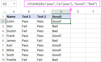
For instance, to output "Good" if both B2 and C2 are greater than 50, "Bad" otherwise, the formula is:
=IF(AND(B2="pass", C2="pass"), "Good!", "Bad")
Important note! The AND function checks all the conditions, even if the already tested one(s) evaluated to FALSE. Such behavior is a bit unusual since in most of programming languages, subsequent conditions are not tested if any of the previous tests has returned FALSE.
In practice, a seemingly correct IF statement may result in an error because of this specificity. For example, the below formula would return #DIV/0! ("divide by zero" error) if cell A2 is equal to 0:
=IF(AND(A2<>0, (1/A2)>0.5),"Good", "Bad")
The avoid this, you should use a nested IF function:
=IF(A2<>0, IF((1/A2)>0.5, "Good", "Bad"), "Bad")
For more information, please see IF AND formula in Excel.
Excel IF function with multiple conditions (OR logic)
To do one thing if any condition is met, otherwise do something else, use this combination of the IF and OR functions:
The difference from the IF / AND formula discussed above is that Excel returns TRUE if any of the specified conditions is true.
So, if in the previous formula, we use OR instead of AND:
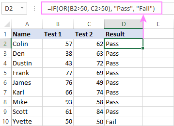
=IF(OR(B2>50, B2>50), "Pass", "Fail")
Then anyone who has more than 50 points in either exam will get "Pass" in column D. With such conditions, our students have a better chance to pass the final exam (Yvette being particularly unlucky failing by just 1 point :)
Tip. In case you are creating a multiple IF statement with text and testing a value in one cell with the OR logic (i.e. a cell can be "this" or "that"), then you can build a more compact formula using an array constant.
For example, to mark a sale as "closed" if cell B2 is either "delivered" or "paid", the formula is:
=IF(OR(B2={"delivered", "paid"}), "Closed", "")
More formula examples can be found in Excel IF OR function.
IF with multiple AND & OR statements
If your task requires evaluating several sets of multiple conditions, you will have to utilize both AND & OR functions at a time.
In our sample table, suppose you have the following criteria for checking the exam results:
- Condition 1: exam1>50 and exam2>50
- Condition 2: exam1>40 and exam2>60
If either of the conditions is met, the final exam is deemed passed.
At first sight, the formula seems a little tricky, but in fact it is not! You just express each of the above conditions as an AND statement and nest them in the OR function (since it's not necessary to meet both conditions, either will suffice):
OR(AND(B2>50, C2>50), AND(B2>40, C2>60)
Then, use the OR function for the logical test of IF and supply the desired value_if_true and value_if_false values. As the result, you get the following IF formula with multiple AND / OR conditions:
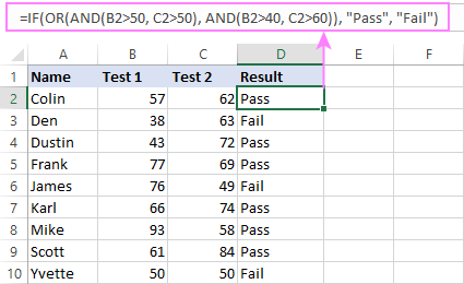
=IF(OR(AND(B2>50, C2>50), AND(B2>40, C2>60), "Pass", "Fail")
The screenshot below indicates that we've done the formula right:
Naturally, you are not limited to using only two AND/OR functions in your IF formulas. You can use as many of them as your business logic requires, provided that:
- In Excel 2007 and higher, you have no more than 255 arguments, and the total length of the IF formula does not exceed 8,192 characters.
- In Excel 2003 and lower, there are no more than 30 arguments, and the total length of your IF formula does not exceed 1,024 characters.
Nested IF statement to check multiple logical tests
If you want to evaluate multiple logical tests within a single formula, then you can nest several functions one into another. Such functions are called nested IF functions. They prove particularly useful when you wish to return different values depending on the logical tests' results.
Here's a typical example: suppose you want to qualify the students' achievements as "Good", "Satisfactory" and "Poor" based on the following scores:
- Good: 60 or more (>=60)
- Satisfactory: between 40 and 60 (>40 and <60)
- Poor: 40 or less (<=40)
Before writing a formula, consider the order of functions you are going to nest. Excel will evaluate the logical tests in the order they appear in the formula. Once a condition evaluates to TRUE, the subsequent conditions are not tested, meaning the formula stops after the first TRUE result.
In our case, the functions are arranged from largest to smallest:
=IF(B2>=60, "Good", IF(B2>40, "Satisfactory", "Poor"))
Naturally, you can nest more functions if needed (up to 64 in modern versions).

For more information, please see How to use multiple nested IF statements in Excel.
Excel IF array formula with multiple conditions
Another way to get an Excel IF to test multiple conditions is by using an array formula.
To evaluate conditions with the AND logic, use the asterisk:
To test conditions with the OR logic, use the plus sign:
To complete an array formula correctly, press the Ctrl + Shift + Enter keys together. In Excel 365 and Excel 2021, this also works as a regular formula due to support for dynamic arrays.
For example, to get "Pass" if both B2 and C2 are greater than 50, the formula is:
=IF((B2>50) * (C2>50), "Pass", "Fail")

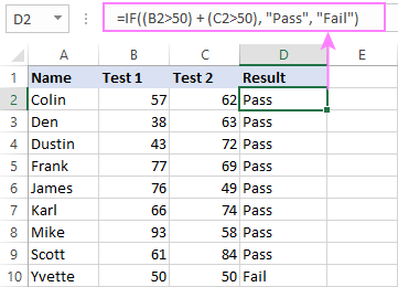
In my Excel 365, a normal formula works just fine (as you can see in the screenshots above). In Excel 2019 and lower, remember to make it an array formula by using the Ctrl + Shift + Enter shortcut.
To evaluate multiple conditions with the OR logic, the formula is:
=IF((B2>50) + (C2>50), "Pass", "Fail")
Using IF together with other functions
This section explains how to use IF in combination with other Excel functions and what benefits this gives to you.
Example 1. If #N/A error in VLOOKUP
When VLOOKUP or other lookup function cannot find something, it returns a #N/A error. To make your tables look nicer, you can return zero, blank, or specific text if #N/A. For this, use this generic formula:
For example:
If #N/A return 0:
If the lookup value in E1 is not found, the formula returns zero.
=IF(ISNA(VLOOKUP(E1, A2:B10, 2,FALSE )), 0, VLOOKUP(E1, A2:B10, 2, FALSE))
If #N/A return blank:
If the lookup value is not found, the formula returns nothing (an empty string).
=IF(ISNA(VLOOKUP(E1, A2:B10, 2,FALSE )), "", VLOOKUP(E1, A2:B10, 2, FALSE))
If #N/A return certain text:
If the lookup value is not found, the formula returns specific text.
=IF(ISNA(VLOOKUP(E1, A2:B10, 2,FALSE )), "Not found", VLOOKUP(E1, A2:B10, 2, FALSE))

For more formula examples, please see VLOOKUP with IF statement in Excel.
Example 2. IF with SUM, AVERAGE, MIN and MAX functions
To sum cell values based on certain criteria, Excel provides the SUMIF and SUMIFS functions.
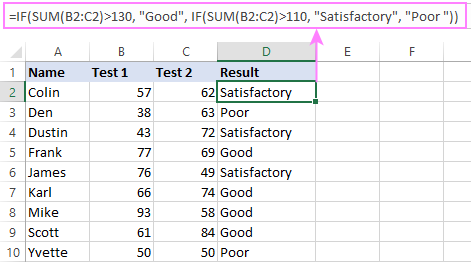
In some situations, your business logic may require including the SUM function in the logical test of IF. For example, to return different text labels depending on the sum of the values in B2 and C2, the formula is:
=IF(SUM(B2:C2)>130, "Good", IF(SUM(B2:C2)>110, "Satisfactory", "Poor"))
If the sum is greater than 130, the result is "good"; if greater than 110 – "satisfactory', if 110 or lower – "poor".
In a similar fashion, you can embed the AVERAGE function in the logical test of IF and return different labels based on the average score:
=IF(AVERAGE(B2:C2)>65, "Good", IF(AVERAGE(B2:C2)>55, "Satisfactory", "Poor"))
Assuming the total score is in column D, you can identify the highest and lowest values with the help of the MAX and MIN functions:
=IF(D2=MAX($D$2:$D$10), "Best result", "")
=IF(D2=MAX($D$2:$D$10), "Best result", "")
To have both labels in one column, nest the above functions one into another:
=IF(D2=MAX($D$2:$D$10), "Best result", IF(D2=MIN($D$2:$D$10), "Worst result", ""))

Likewise, you can use IF together with your custom functions. For example, you can combine it with GetCellColor or GetCellFontColor to return different results based on a cell color.
In addition, Excel provides a number of functions to calculate data based on conditions. For detailed formula examples, please check out the following tutorials:
Example 3. IF with ISNUMBER, ISTEXT and ISBLANK
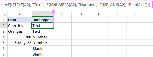
To identify text, numbers and blank cells, Microsoft Excel provides special functions such as ISTEXT, ISNUMBER and ISBLANK. By placing them in the logical tests of three nested IF statements, you can identify all different data types in one go:
=IF(ISTEXT(A2), "Text", IF(ISNUMBER(A2), "Number", IF(ISBLANK(A2), "Blank", "")))
Example 4. IF and CONCATENATE
To output the result of IF and some text into one cell, use the CONCATENATE or CONCAT (in Excel 2016 - 365) and IF functions together. For example:
=CONCATENATE("You performed ", IF(B1>100,"fantastic!", IF(B1>50, "well", "poor")))
=CONCAT("You performed ", IF(B1>100,"fantastic!", IF(B1>50, "well", "poor")))
Looking at the screenshot below, you'll hardly need any explanation of what the formula does:

IF ISERROR / ISNA formula in Excel
The modern versions of Excel have special functions to trap errors and replace them with another calculation or predefined value - IFERROR (in Excel 2007 and later) and IFNA (in Excel 2013 and later). In earlier Excel versions, you can use the IF ISERROR and IF ISNA combinations instead.
The difference is that IFERROR and ISERROR handle all possible Excel errors, including #VALUE!, #N/A, #NAME?, #REF!, #NUM!, #DIV/0!, and #NULL!. While IFNA and ISNA specialize solely in #N/A errors.
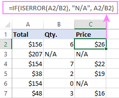
For example, to replace the "divide by zero" error (#DIV/0!) with your custom text, you can use the following formula:
=IF(ISERROR(A2/B2), "N/A", A2/B2)
And that's all I have to say about using the IF function in Excel. I thank you for reading and hope to see you on our blog next week!
Practice workbook for download
Excel IF multiple criteria - examples (.xlsx file)
 by
by
4506 comments
Hey,
I have searched everywhere to find the correct conditions for my IF function formula. Please help!
If the cell value is over $50,000 but not over $75,000, add $7,500 plus 25% of the amount over $50,000. I need the range to be over $50,000 but not over $75,000.
For Example:
If the cell value is 60,000, I need the formula to add $7,500 plus (excess amount over $50,000)*25% [7500+(60000-50000)]
Hi!
If my understanding of the task is correct, the following formula should work a treat:
=IF(AND(A1>50000, A1<75000), 7500+(A1-50000)*25%, "")
How can I get this type of formula to work? I am trying to get a value if criteria are met in two cells that comprise of multiple drop down list values.
=OR((((IF(AND(C2=1,D2="Towers"),"Nito",""),IF(AND(C2=1,D2="A-Pick"),"Nito",""),IF(AND(C2=2,D2="Towers"),"Angeline","")))))
Hi Svetlana,
What do the quotation marks in the formula below stand for?
=IF(L23="","",(L23-$L$31)^2)
Thank you.
Steve
Hi Stephen,
"" stands for an empty string, i.e. a blank cell.
So, the formula reads as follows: if L23 is empty (or contains an empty string returned by some other formula), then return nothing (blank cell), otherwise return the result of the calculation.
IF Column A anything equal to Column B then select the value from column C corresponding to Column B.
I have two different dates in Column A and Column B and want to match them and after matching select the value from Column C corresponding to Column B
Hi!
Unfortunately, I can't understand what you want to do. Explain what it means to "compare two different dates" and "select the value from Column C corresponding to Column B".
Hi,
Is someone able to help me please, i'm trying to work out how to get different values based on day parameters, for example starting with 30 June, day 1 to 7 is charged at $75 a day, then day 8 to 14 is charged at $105, then any days from day 15 is then charged at $135, so i'm trying to based on the number of days charged, bring across the right day charge based on the day parameter.
All this is from one line in excel.
Hope you can help.
Thanks
Chantelle
Thank you Svetlana
I have another question. I have a vlookup that is wrapped around an IFERROR function. So when there is an error the cell returns blank. Now I need to have conditional formatting on that blank cell. What is the rule with reference to that cell. Using the cell value is equal to blank or N/A doesn't seem to work. Can you provide some expertise?
thanks again
Hi Michelle,
You can create a rule with the formula like =$B2="" where B2 is the top-most cell with your IFERROR/VLOOKUP formula.
hi is someone able to help with the following:
I have a date format in one cell (CQ)that appears like this 2015/07/24 and I would like to link an IF formula to that date cell. The intention is if the CQ date cell has a date in it (numeric) return the date in tact. And if the same CQ cell contains nothing (blank) return blank "". I am using the following formula but it isn't working:
=IF(CQ7="numeric",CQ7,"")
Unfortunately it doesn't like number, date or numeric. What can I put in the spot of "numeric" that will make this formula work?
thank you in advance
Hi Michelle,
Excel has a special function, ISNUMBER, to identify numeric values. So, you can write the formula as follows:
=IF(ISNUMBER(CQ7), CQ7, "")
Please note that it returns a serial number representing the date and to force it to appear as a date, you need to apply the Date format to the cell with the above formula.
I am trying to find a relatively simple (I hope) formula for a time sheet.
Column C is the Start Time
Column E is the End Time.
Colmun F would be the total hours worked.
I have worked out =sum(E3-C3)/100-0.3
What I need is to equate "OFF" and "LV" to 0 in F3.
Thanks in advance!
Hi Nicole,
Sorry, I am not sure I understand the task. Do you enter that formula in F3 and want it to display "OFF" or "LV" when the formula returns 0? Please clarify.
Hi I am wondering what the underlying is in the following formula:
=IFERROR(VLOOKUP(B6,'Asset Mix'!W:GR,178,FALSE),"")
Without the "" at the end of the formula, it would return #N/A. I am trying to link a formula in another cell to the blank cell in the formula above, but it won't accept the "" as a blank - what is really in this cell?
Hi Svetlana
Could you please help me with the below.
I would like to have one cell with following two formulas:
=D43*H20
But also:
=IF(E43="","","D43*H20")
So if E43 is blank then the cell is blank and if it is not blank then it contains the formula D43*H20
Is this possible?
Thanks so much
Luke
Hi Samuel,
You were almost there :) Just remove the quotation marks enclosing the formula in the last argument:
=IF(E43="","", D43*H20)
Hi
I am stuck in a situtation where I have multiple excel sheet and I am trying to generate a summery sheet which gives me quick detail here but not able to move ahead. Let me explain what I am looking for: I have various locations where some sales activities will keep on happening everymonth. Now I want to know how many activities happen in a period of 1 month in a particular area. The complexity is that in other sheet the same area is mentioned several times as dates may differ.
Now I want that in the summary sheet, I should get that area to be mentioned once and no. of activities happened in that area in the entire month.
Please help!
Gostei! Foi pra mim muito util!
I have this problem;
When the value from a cell in column A is different to the value in the cell below, use column C otherwise use column B. Now if the value in column C is greater then 1000000 default the value to 1000000 and if it’s less then 0 default it to 0.
My Solution:
=IF(A1A2, IF(C1>100000, 100000, 0),B1)
Please help me get correct results
=IF(AND(I20="Non-US", E20>E13), "XS1261825977", "N/A"), IF(AND(I20="Accredited Investor", E20>E13), "XS1261826512", "N/A"), IF(AND(I20="QIB", E20>E13), "XS1261826512", "N/A"), IF(AND(I20="Non-eligible", E20>E13), "N/A", "N/A")
E20>E13 is simply checking that a numerical amount is higher than another.
Hello.
is there aything immediately obvious with the above formula?
is it OK to nest IF(AND) like this?
I am getting the #VALUE! error.
Hi team, I have been reading through the article and all comments attempting to solve for a broken formula, so I am hoping I can call upon your collective brain cells to solve for this.
I am trying to determine if a document was created before or after a certain date, pulling from an array of data. My formula (and I don't know what I'm doing wrong here), looks like this:
=IF((AND(ENCOUNTERS!D:D,"="&B5,ENCOUNTERS!G:G,">"&C5)),"YES","NO")
I'm getting a #VALUE error within the cell.
Data within B5 is an ID number
Data within Encounters!D:D is a list of ID numbers
Data within C5 is the specific date in question
Data within Encounters!G:G is a date corresponding to the ID number
I think my edrror has something to do with the fact that I'm working with dates, but I am uncertain. Any feedback would be dearly appreciated.
When I concatenate 2 date columns and display, I use the formula
=TEXT([A1],"mm/dd")&" - "&TEXT([B1],"mm/dd")
I need to add an additional condition , If either A1 or B1 or both are empty , nothing should be concatenated and displayed.
=IF(OR(AND(A1="", B1=""), AND(A1="")), ,( TEXT([A1],"mm/dd")&" - "&TEXT([B1],"mm/dd")))
I wonder is this will work. Any help is appreciated.
Hey,
I have searched everywhere to find the correct conditions for my IF function formula. Please help!
If the cell value is over $50,000 but not over $75,000, add $7,500 plus 25% of the amount over $50,000. I need the range to be over $50,000 but not over $75,000.
For Example:
If the cell value is 60,000, I need the formula to add $7,500 plus (excess amount over $50,000)*25% [7500+(60000-50000)]
Hey
"In cell J9, use a function to display the name, school and symbol of the top student as such Smith, A from Cape High School scored A."
for this question what function can I use to consolidate name, school and grade of the top student?
IF
functions
which
returns
NO
NEED
or
SEND
NOW
or
CHECK
IT
IN
TWO
WEEKS
A B (Values) C(Answer)
MISJ 5000 5000
DIV 500 500
MISJ 1500 1500
JV 1000 0
Please help me to develop formula for above calculation
I need " MISJ"and "DIV" values in C column
Hi Nandana,
Here's the formula for C1:
=IF(OR(A1="misj", A1="div"), B1, 0)
I have sets of data, for example like this
Sam Bella Sara Adam
Modal $1,000 $2,000 $3,000 $1,000
Work Order Cost
Sam, Adam $100
Bella, Sara, Adam $200
I need to divide the value of 'cost' to the respective individu. For example, 'cost' $100. I want this value divide evenly to Sam and Adam based on their respective modal value . So the calculation supposedly, ($100x$1000)/($1000+$1000) = $50. Same goes with Adam since their modal value is same.
So I want a formula which can capture the names and return the value needed in the calculation.
Please assist me to solve this. Thanks.
if A1=blanck (no value) then B2 (where the curser is)should be blank
if A1 is "not like" "ES/*" then B2 NM
Pl let me know the formula
In excel file I have 5 coloums with different name.
In another excel file I have 100 rows with 2 coloums.
In one coloumn there is amount and another coloumn there is names which is there in 1st excel file
please suggest a formula through which I can sum the amount from 2nd excel sheet to 1st excel sheet according to the name.
This was incredibly helpful. Excellent article. Thank you!
Dear Svetlana,
I am also trying to learn some of the insides. Please help with the following: let's say I have 10 products with a cost of 1,2,3,4,5..10Eur. In order to find a sale price I want to put them in categories: from 1-4,5-7,8-10. Each category has a different percentage added: 1-4: 200%; 5-7: 150%; and 8-10: 100%.
How can I link a formula to automatically multiply the purchase cost with the right percentage?
Thank you!
Hi,
I am trying to write formula for the following condition in my work sheet but I am unable to write can I get help?
condition : first condition if(c2=1) and count(P2:R2)=0,then "OD", "OT" ) or if(c2=2) and count (M2:R2)=0, then"OD", "OT" )
Hi,
I'm looking for a formula that could be used like this:
Year number : 1 - 30
Tables x, y, z the number of purchases made in table x which is in euros, the number of purchases made in table y in francs, and the number of purchases made in dollars.
If I chose year 6 it will give me a value in tables x. THEN IF I wish to chose year 19 it will give me another value in table x. How do I make this formula as I write in the number? Thanks!
Hello,
This formula works: =ROUND(IF($E5="MCP",$V5*Rates!B$3,0),2) and this works: =ROUND(IF($E5="CWA",$V5*Rates!B$4,0),2) but I want them be together in the same formaula...multiple conditions. For some reason, today, I am just drawing a blank and am having trouble combining the two.
Note: Rates!B$3 = 3% and Rates!B$3 = 4% and $E5 is a dollar amount
Thank you.
Never mind. I got. :-)
Hi there
What formula do i use to get correct result for:-
if Cell A2 contains "ABC" and B2 cell contains "100%" then i want C2 cell shows "OK" & if Cell A2 contains "DEF" and B2 cell contains ">=50" then i want C2 cell shows "OK" & if Cell A2 contains "XYZ" and B2 cell contains ">=35%" then i want C2 cell shows "OK" otherwise C2 shows "Pending"
Like below:-
Pocedure Result Process
ABC 100% OK
DEF 50% OK
XYZ 35% OK
ABC 90% Pending
XYZ 35% OK
DEF 40% Pending
ABC 75% Pending
XYZ 10% Pending
Very informative Site: i am having a problem please solve it out, Thanks.
I want Result in a certain cell: if Value in E3 is above 400000 but less than 750000, then (E3-400000) x 5% and add zero, but if value is greator than 750000 but less than 1400000, then (E3-750000) x 10%+17500, i am unable to figure it out,
Please help
I am using this formula. IF((AND(E3>=400000,E3=750000,E3<1400000),(E3-750000)*10%+17500),0)
Hi,
What formula can I use to assign if the particular time is of AM or PM shift? Here's the scenario:
AM shift falls within 8:00 AM to 19:59 PM
PM shift falls within 20:00 PM to 7:59 AM
However, cell value is in date and time, while above are of time value only.
Thanks!
=IF(OR(ISNUMBER(SEARCH("Top 25%",E9)),ISNUMBER(SEARCH("Top 50%",E9))*ISNUMBER(SEARCH("Bottom 50%",E9))),"12","8")
In the above formula I want "Bottom 50%" to be 4. if I am adding 4 after eight in formula. I get error .
Please help
Can someone assist me. I have the following criteria I have a range of cells from F4:F14 where some cells have text and the others have numbers.
What I need to accomplish:
Pass if cell value F4 is 0.1 or higher
Pass if cell value F4 has any text
Fail if cell value F4 is equal to 0
then I need to display (Pass / Fail) in cell F15 which is the total of F4:F14
Hello
Could you please help me with the following formula:
If a cell (date of booking) is blank then 0 or if the cell ( date of booking )> another cell (date of enquiry) then also 0 otherwise 1.
Thank you
Hi,
I want to report a result =0.05 in one digit. Is it possible with 'IF' condition.
Regards
Kumar swamy
if, 1)for 0 to 250000 ,tax is 0%
2)for 250000 to 500000 tax is 10%
3)for 500000 to 1000000 tax is20%
for 1000000 to above tax 30%
e.g.,if taxable income is 650000 then tax will be
for 1) for 250000x0%=0
2) for 250000x10%= 25000
3) for 150000x20%=30000
so, total tax = 55000
what will be the formula
Hi Svetlana,
I hope you can help me I really need your assistance on this. I am working on a time sheet where I am trying to execute the following:
(time out-time in)-meal break time. The output will go into the column "regular time". That is no problem and easily accomplished. The hitch is I want the output to go to the column "vacation time" if the block in the column "Vacation day" has a Y in in it. To summarize I am trying to get:
"(Time out-Time in)-Meal break=regular time, if Vacation day="Y" then (Time out-Time in)-Meal break=Vacation time."
I hope this makes sense and I really appreciate the assistance!!
Thank you in advance for the help!!
Kind regards,
Raymond
HI,
I could also use some assistance with another formula. I would like to sum the values from FX:GE to get a total score, but if the total score = 16, I would like it say "-1" instead. Is this possible?
Thanks!
Hi Courtney,
Here you go:
=IF(SUM(FX1:GE100)=16,-1,SUM(FX1:GE100))
Hi Svetlana,
Thank you for all of your support on this amazing website! I would appreciate your help making one If/then statement for the following:
If GI = 8, then "-1"
If GF = 8, then "1"
If GF + GG = 8, then "2"
If GH + GI = 1 or 2, then "3"
If GH + GI = 3 or 4, then "4"
If GH + GI > 4, then "5"
Thank you!
Hi Courtney,
Here's the formula as per your conditions:
=IF(GI1=8,-1, IF(GF1=8,1, IF(GF1+GG1=8,2, IF(OR(GH1+GI1=1,GH1+GI1=2),3, IF(OR(GH1+GI1=3,GH1+GI1=4),4, IF(GH1+GI1>4,5,""))))))
Please keep in mind that nested IF formulas elevate the first condition first and if it's met, other conditions are not tested. For example, if GI1=8, the formula will always return -1 regardless of the values in other cells.
Hi, so I'm trying to compare two values but they are not integers. How can I do this?
Condition: If A1 is "High" and B2 is "Low", C1 should be "Q1". This would be different if A1 is Low and B2 is High, it will print "Q2" and so on. IS this possible?
Hi Ivan,
Of course this is possible with the following formula:
=IF(AND(A1="high",B2="low"),"Q1",IF(AND(A1="low",B2="high"),"Q2",""))
Good afternoon,
I am working on a time sheet where I am trying to execute the following:
(time out-time in)-meal break time. The output will go into the column "regular time". That is no problem and easily accomplished. The hitch is I want the out to go to the column "vacation time" if the block in the column "Vacation day" has a Y in in it. To summarize I am trying to get:
"(Time out-Time in)-Meal break=regular time, if Vacation day="Y" then (Time out-Time in)-Meal break=Vacation time."
I hope this makes sense and I really appreciate the assistance!!
Thank you in advance for the help!!
Kind regards,
Raymond
Svetlana,
Hi! I have a spreadsheet that I am using to calculate a certain ratio. A lot of times it will come back with a null value which is what I want. Formula is: =IFERROR(AR416/H416,"")
But, there are times where the value comes to $0.00 which unfortunately gets pulled into my AVERAGEIFS formula and pulls down the average considerably.
So I tried this formula to counteract that:
=IF(AR419/H419>0,IFERROR(AR419/H419,""),"")
But now I get the divide by zero error in a few cells: #DIV/0!.
Is there a way to use an IF statement to return a null value for everything that isn't greater than 0?
Thanks so much!
Shawn
Perfect! Thanks so much for your help Svetlana!
Hi WENDY,
Try this one:
=IF(AND(R1126>10.1,S1126>2.1),"TF2", IF(R1126>=10.1,"TF1", IF(S1126>=6.1, 3, IF(S1126>=2.1, 2,IF(S1126<=2,1)))))
Hi! I am trying to add one more equation to my IF function and am not sure what to do. Here is my equation so far: =IF(R1126>=10.1,"TF1",IF(S1126>=6.1,"3",IF(S1126>=2.1,"2",IF(S1126<=2,"1")))) What I also need it to do is come back with a posting of TF2 if R1126 is greater than 10.1 AND S1126 is greater that 2.1. I cannot figure out what I am doing wrong. Any suggestions?
Hi
Can you help me with why this function is giving invalid errors? My error starts at this statement:IF(B43="",IF(A43=TODAY(),("OTW"),("CHECK ETA"))
and again at this statement:IF(G43="",("IN ROUTE"),IF(L43"",("DELIVERED"),IF(H43="",("NOT AVAIL"),IF(I43"",("SCHEDULED"),("NEEDS SCHEDULED")))
=IF(F43="",IF(A43>=TODAY(),("OTW"),IF(B43="",("CHECK ETA"),("ARRIVED")),IF(B43="",IF(A43=TODAY(),("OTW"),("CHECK ETA")),IF(D43="",IF(B43"",("AT PORT"),("OTW")),IF(E43="",IF(D43"",("INGATED"),IF(B43"",("AT THE PORT"),("OTW")),IF(G43="",("IN ROUTE"),IF(L43"",("DELIVERED"),IF(H43="",("NOT AVAIL"),IF(I43"",("SCHEDULED"),("NEEDS SCHEDULED")))
Hi Svetlana
How ican convert the currency value to USD if the available currency is anything else say , in 1 row (A:A) I have AED, Pounds, Euro, RS and they should be converted to USD in another ROW (B).
1 more point is for the convenience in Row B we can see what currency has hadded. Like A1: 100 B1: Eur and in C1 : I have to have A1 value in USD here. We have standard conversion value.usd to Eur is 1.09 and for AED to USD is 3.67. so n so.
Regards
Rajesh
I have several false and true statements across a row. I want to make one formula that says if all statements are false, give me false. If one is true, give me true.
Hi Sarah,
You can use a formula similar to this:
=IF(COUNTIF(A1:E1, TRUE)>0, TRUE, FALSE)
i have a query on the below data...
i have max value and min sale value..
i have value for march sale.
if my sale is gone beyond max value upto 25%, then should be zero, or between the max value then it should be show some points based upon or will calculate in 10.
The same is required for min value too...but i want to use both condition in one single column.
Pls help.quite urgent for me.
Hi, I am trying to do an IF function with two text variables. If the other cell says either SLEEVE or FLANGE, then the IF cell returns a 1. I can't figure it out for Excel 2013. Help! :)
Hi Nick,
What you need is a OR statement like this:
=IF(OR(A1="SLEEVE", A1="FLANGE"), 1, "")
And what do you add to the formula if it must leave the cell blank is nothing is entered in the column yet? I want the number 2 to be returned if any other word is typed in, but I need the cell to be blank if I did not type something in. Eg
=IF(OR(A1="SLEEVE",A1="FLANGE"),1,2)
Hi Vinette,
In this case, nest another If function, like this:
=IF(OR(A1="SLEEVE",A1="FLANGE"),1, IF(A1<>"",2,""))
Hi
My data is as below,
If a cell says something else apart from shipped , then the other cell has to count the due days from today date to an already specified date (say acknowledged date).Which formula suits best for that.
i.e. If S12 is not equal to "Shipped" then count Today-acknowledged (Q12). the result should be in days.
Regards
Rajesh
Hi Rajesh,
Try this formula:
=IF(S12<>"shipped", TODAY()- Q12, "")
Worked. GREAT!!! Thank you Svetlana.
How ican convert the currency value to USD if the available currency is anything else say , in 1 row (A:A) I have AED, Pounds, Euro, RS and they should be converted to USD in another ROW (B).
1 more point is for the convenience in Row B we can see what currency has hadded. Like A1: 100 B1: Eur and in C1 : I have to have A1 value in USD here. We have standard conversion value.usd to Eur is 1.09 and for AED to USD is 3.67. so n so.