The tutorial shows how to create multiple IF statements in Excel with AND as well as OR logic. Also, you will learn how to use IF together with other Excel functions.
In the first part of our Excel IF tutorial, we looked at how to construct a simple IF statement with one condition for text, numbers, dates, blanks and non-blanks. For powerful data analysis, however, you may often need to evaluate multiple conditions at a time. The below formula examples will show you the most effective ways to do this.
How to use IF function with multiple conditions
In essence, there are two types of the IF formula with multiple criteria based on the AND / OR logic. Consequently, in the logical test of your IF formula, you should use one of these functions:
- AND function - returns TRUE if all the conditions are met; FALSE otherwise.
- OR function - returns TRUE if any single condition is met; FALSE otherwise.
To better illustrate the point, let's investigate some real-life formulas examples.
Excel IF statement with multiple conditions (AND logic)
The generic formula of Excel IF with two or more conditions is this:
Translated into a human language, the formula says: If condition 1 is true AND condition 2 is true, return value_if_true; else return value_if_false.
Suppose you have a table listing the scores of two tests in columns B and C. To pass the final exam, a student must have both scores greater than 50.
For the logical test, you use the following AND statement: AND(B2>50, C2>50)
If both conditions are true, the formula will return "Pass"; if any condition is false - "Fail".
=IF(AND(B2>50, B2>50), "Pass", "Fail")
Easy, isn't it? The screenshot below proves that our Excel IF /AND formula works right:

In a similar manner, you can use the Excel IF function with multiple text conditions.
For instance, to output "Good" if both B2 and C2 are greater than 50, "Bad" otherwise, the formula is:
=IF(AND(B2="pass", C2="pass"), "Good!", "Bad")
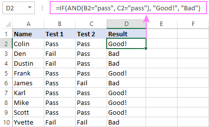
Important note! The AND function checks all the conditions, even if the already tested one(s) evaluated to FALSE. Such behavior is a bit unusual since in most of programming languages, subsequent conditions are not tested if any of the previous tests has returned FALSE.
In practice, a seemingly correct IF statement may result in an error because of this specificity. For example, the below formula would return #DIV/0! ("divide by zero" error) if cell A2 is equal to 0:
=IF(AND(A2<>0, (1/A2)>0.5),"Good", "Bad")
The avoid this, you should use a nested IF function:
=IF(A2<>0, IF((1/A2)>0.5, "Good", "Bad"), "Bad")
For more information, please see IF AND formula in Excel.
Excel IF function with multiple conditions (OR logic)
To do one thing if any condition is met, otherwise do something else, use this combination of the IF and OR functions:
The difference from the IF / AND formula discussed above is that Excel returns TRUE if any of the specified conditions is true.
So, if in the previous formula, we use OR instead of AND:
=IF(OR(B2>50, B2>50), "Pass", "Fail")
Then anyone who has more than 50 points in either exam will get "Pass" in column D. With such conditions, our students have a better chance to pass the final exam (Yvette being particularly unlucky failing by just 1 point :)
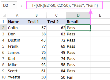
Tip. In case you are creating a multiple IF statement with text and testing a value in one cell with the OR logic (i.e. a cell can be "this" or "that"), then you can build a more compact formula using an array constant.
For example, to mark a sale as "closed" if cell B2 is either "delivered" or "paid", the formula is:
=IF(OR(B2={"delivered", "paid"}), "Closed", "")
More formula examples can be found in Excel IF OR function.
IF with multiple AND & OR statements
If your task requires evaluating several sets of multiple conditions, you will have to utilize both AND & OR functions at a time.
In our sample table, suppose you have the following criteria for checking the exam results:
- Condition 1: exam1>50 and exam2>50
- Condition 2: exam1>40 and exam2>60
If either of the conditions is met, the final exam is deemed passed.
At first sight, the formula seems a little tricky, but in fact it is not! You just express each of the above conditions as an AND statement and nest them in the OR function (since it's not necessary to meet both conditions, either will suffice):
OR(AND(B2>50, C2>50), AND(B2>40, C2>60)
Then, use the OR function for the logical test of IF and supply the desired value_if_true and value_if_false values. As the result, you get the following IF formula with multiple AND / OR conditions:
=IF(OR(AND(B2>50, C2>50), AND(B2>40, C2>60), "Pass", "Fail")
The screenshot below indicates that we've done the formula right:
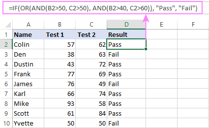
Naturally, you are not limited to using only two AND/OR functions in your IF formulas. You can use as many of them as your business logic requires, provided that:
- In Excel 2007 and higher, you have no more than 255 arguments, and the total length of the IF formula does not exceed 8,192 characters.
- In Excel 2003 and lower, there are no more than 30 arguments, and the total length of your IF formula does not exceed 1,024 characters.
Nested IF statement to check multiple logical tests
If you want to evaluate multiple logical tests within a single formula, then you can nest several functions one into another. Such functions are called nested IF functions. They prove particularly useful when you wish to return different values depending on the logical tests' results.
Here's a typical example: suppose you want to qualify the students' achievements as "Good", "Satisfactory" and "Poor" based on the following scores:
- Good: 60 or more (>=60)
- Satisfactory: between 40 and 60 (>40 and <60)
- Poor: 40 or less (<=40)
Before writing a formula, consider the order of functions you are going to nest. Excel will evaluate the logical tests in the order they appear in the formula. Once a condition evaluates to TRUE, the subsequent conditions are not tested, meaning the formula stops after the first TRUE result.
In our case, the functions are arranged from largest to smallest:
=IF(B2>=60, "Good", IF(B2>40, "Satisfactory", "Poor"))
Naturally, you can nest more functions if needed (up to 64 in modern versions).

For more information, please see How to use multiple nested IF statements in Excel.
Excel IF array formula with multiple conditions
Another way to get an Excel IF to test multiple conditions is by using an array formula.
To evaluate conditions with the AND logic, use the asterisk:
To test conditions with the OR logic, use the plus sign:
To complete an array formula correctly, press the Ctrl + Shift + Enter keys together. In Excel 365 and Excel 2021, this also works as a regular formula due to support for dynamic arrays.
For example, to get "Pass" if both B2 and C2 are greater than 50, the formula is:
=IF((B2>50) * (C2>50), "Pass", "Fail")

In my Excel 365, a normal formula works just fine (as you can see in the screenshots above). In Excel 2019 and lower, remember to make it an array formula by using the Ctrl + Shift + Enter shortcut.
To evaluate multiple conditions with the OR logic, the formula is:
=IF((B2>50) + (C2>50), "Pass", "Fail")
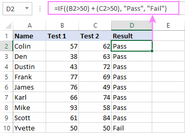
Using IF together with other functions
This section explains how to use IF in combination with other Excel functions and what benefits this gives to you.
Example 1. If #N/A error in VLOOKUP
When VLOOKUP or other lookup function cannot find something, it returns a #N/A error. To make your tables look nicer, you can return zero, blank, or specific text if #N/A. For this, use this generic formula:
For example:
If #N/A return 0:
If the lookup value in E1 is not found, the formula returns zero.
=IF(ISNA(VLOOKUP(E1, A2:B10, 2,FALSE )), 0, VLOOKUP(E1, A2:B10, 2, FALSE))
If #N/A return blank:
If the lookup value is not found, the formula returns nothing (an empty string).
=IF(ISNA(VLOOKUP(E1, A2:B10, 2,FALSE )), "", VLOOKUP(E1, A2:B10, 2, FALSE))
If #N/A return certain text:
If the lookup value is not found, the formula returns specific text.
=IF(ISNA(VLOOKUP(E1, A2:B10, 2,FALSE )), "Not found", VLOOKUP(E1, A2:B10, 2, FALSE))

For more formula examples, please see VLOOKUP with IF statement in Excel.
Example 2. IF with SUM, AVERAGE, MIN and MAX functions
To sum cell values based on certain criteria, Excel provides the SUMIF and SUMIFS functions.
In some situations, your business logic may require including the SUM function in the logical test of IF. For example, to return different text labels depending on the sum of the values in B2 and C2, the formula is:
=IF(SUM(B2:C2)>130, "Good", IF(SUM(B2:C2)>110, "Satisfactory", "Poor"))
If the sum is greater than 130, the result is "good"; if greater than 110 – "satisfactory', if 110 or lower – "poor".
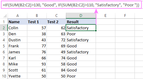
In a similar fashion, you can embed the AVERAGE function in the logical test of IF and return different labels based on the average score:
=IF(AVERAGE(B2:C2)>65, "Good", IF(AVERAGE(B2:C2)>55, "Satisfactory", "Poor"))
Assuming the total score is in column D, you can identify the highest and lowest values with the help of the MAX and MIN functions:
=IF(D2=MAX($D$2:$D$10), "Best result", "")
=IF(D2=MAX($D$2:$D$10), "Best result", "")
To have both labels in one column, nest the above functions one into another:
=IF(D2=MAX($D$2:$D$10), "Best result", IF(D2=MIN($D$2:$D$10), "Worst result", ""))

Likewise, you can use IF together with your custom functions. For example, you can combine it with GetCellColor or GetCellFontColor to return different results based on a cell color.
In addition, Excel provides a number of functions to calculate data based on conditions. For detailed formula examples, please check out the following tutorials:
Example 3. IF with ISNUMBER, ISTEXT and ISBLANK
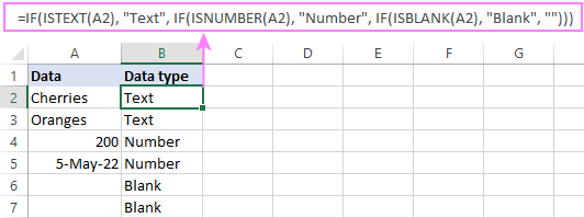
To identify text, numbers and blank cells, Microsoft Excel provides special functions such as ISTEXT, ISNUMBER and ISBLANK. By placing them in the logical tests of three nested IF statements, you can identify all different data types in one go:
=IF(ISTEXT(A2), "Text", IF(ISNUMBER(A2), "Number", IF(ISBLANK(A2), "Blank", "")))
Example 4. IF and CONCATENATE
To output the result of IF and some text into one cell, use the CONCATENATE or CONCAT (in Excel 2016 - 365) and IF functions together. For example:
=CONCATENATE("You performed ", IF(B1>100,"fantastic!", IF(B1>50, "well", "poor")))
=CONCAT("You performed ", IF(B1>100,"fantastic!", IF(B1>50, "well", "poor")))
Looking at the screenshot below, you'll hardly need any explanation of what the formula does:

IF ISERROR / ISNA formula in Excel
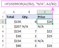
The modern versions of Excel have special functions to trap errors and replace them with another calculation or predefined value - IFERROR (in Excel 2007 and later) and IFNA (in Excel 2013 and later). In earlier Excel versions, you can use the IF ISERROR and IF ISNA combinations instead.
The difference is that IFERROR and ISERROR handle all possible Excel errors, including #VALUE!, #N/A, #NAME?, #REF!, #NUM!, #DIV/0!, and #NULL!. While IFNA and ISNA specialize solely in #N/A errors.
For example, to replace the "divide by zero" error (#DIV/0!) with your custom text, you can use the following formula:
=IF(ISERROR(A2/B2), "N/A", A2/B2)
And that's all I have to say about using the IF function in Excel. I thank you for reading and hope to see you on our blog next week!
Practice workbook for download
Excel IF multiple criteria - examples (.xlsx file)
 by
by
4506 comments
Good evening to the Community!
Would really appreciate if someone can help. I've read every post and made lots of intents, but I am not capable to nest two IF functions. Each works separately
My case is:
I have to get a value in cell cell Q36 of my spreadsheet.
First I have to do: IF(P36<0;(P36+(SUM(Q18:Q23))/60);0), but if the test is false I want to get the result of the following formula, instead of the 0:
IF(Q127<-20000;(SUM($F18:P23)+SUM(Q18:Q23))/60;0)
Can anyone please help?
Not sure if this formula is possible, but I need help trying to create a formula that will cover all four of these possibilities-
If V2 is less than 0 or greater than 1 or less than 241 it equals 1
If V2 is greater than 241 it equals 3
If V2 is equal to 0 and Z2 is also equal to "Done" they equal 2
V2 is equal to 0 and Z2 is also equal to "Pend" or "Sent" they equal 3
If first cell gatter than or less than second cell and when i type pc or rc then 4th cell showing 50% and if i not type pc or rc then it showing 33%
this has me going around in circles.
if column b3 has "yes", column c3 has "yes", column d3 has "Yes" put word "complete" in column g.
i though it would be easy enough but keep getting error. any advice would be appreciated. TIA
I want > 2 cells counta as a one for marking fillup. example
cell- A1=Y & B1=Y than count as a one
or
A1=Y & B1= blank/null or A1=blank/null & B1=Y, than count also as a one
and if both cells show as blank/null than not count
please help me
Hello, I'm trying to write a formula to test a field of options in the test range.
=IF(J13:L29=-1,"(1)","N/A") - so far I'm not getting any luck. Any suggestions?
Hello,
I am trying to get a formula together in order to find the difference in time between two cells. The cells look like this for example:
Target date Start Date
03/05/2019 07:37 03/05/2019 10:26
I need a formula that dates in consideration not only the date but the time as well as if it at any point it is over 24 hours it would be classed as a "fail"
Can anyone help?
Hello
I'm trying to write a formula that has 3 if's and an addition of another cell:
If B5<5 then multiply by B10, if B5 is between 5-10 then multiply by C10, if B5 is 31< then multiply by D10, then add B7
I seem to be able to get one or another to work but I can't get all 3 ifs to work. Some advice on this would be appreciated.
Hi everyone, appreciate if you can assist.
How to write a formula in excel based on the requirement as follows:
First scenario:
IF ≤ 40 KM, rate applies is 60 cents per KM ; and
IF >40 KM, rate applies is 50 cents per KM.
Second scenario
IF ≤ 40KM and/or >40KM, rates is fixed at constant 4o cents per KM.
appreciate your feedback soonest. Thank you.
Hi...!
Here is my query.
For example "B32" cell equals to "FALSE" then find the difference between "B31 and C31".
Please answer my query ?
Hi, please can you help me - is it possible for one cell's value to cancel the formula in another cell? eg - ive got column e which has an expiry date formula (if a tender is not submitted by a particular date, then the cell turns red), but I want to add a column g for submitted YES / NO. What I want to do, is that if the estimator selects yes, then the formula in column e is cancelled / overwritten so that it does not change red anymore- this would be great ... but if I could go one step further, i would like to add a column for the date submitted, and i would like it to function that column g cannot be changed to YES, if the date on which the tender was submitted, hasn't been entered into column h. is this even possible? Thank you in advance for any assistance in this regard.
How do you manage to close a bracket that has not been opened?!
HI!
I am creating a trucking calculator in which the user enters a weight, and the amount to pay the trucker is displayed. The user selects the town from a drop down list, and it calculates the rate depending on the town.
I have a VLOOKUP table which lists the towns and their rates. There are only 2 rates which are divided into zones (1 and 2), and a "Special" rate which will only show the word special. The columns in the VLOOKUP is:
Column 1: town name,
Column 2: rate
Column 3: either the number 1,or 2 (which classifies the towns into 2 zones), or the word "Special".
so far I have the calculator showing the rate once the weight is entered, and the town selected. or the word "Special" if it is a special rate:
=IF(I8="SPECIAL", "SPECIAL", D4*I8)
Now I want to use MAX because there are minimum fees associated. So if the value that is calculated in E13 is less than 26.25, it will display 26.25 instead of the total.
now, the minimum in zone 1 (26.25) is different that zone 2 (29.40).
I need to create a formula that can identify what zone is being used, which can be identified by the number 1, or 2 in cell K8, and apply that minimum charge depending on it.
Need Help
We have 5 Warehouses.
If 3 or more warehouses have 1 or greater value then put "In Stock" else "Out of Stock".
Is it possible?
I have a multi-sheet document and need help writing this expression. The information on sheet2 B column does not change while the f column may change occasionally.
If b2=Sheet2!b:b and D1=sheet2!f:f then ”x” else blank
Thanks in advance
I have the list of students comes from three classes,4A,4B AND 4C,I want to use countif and put total number of students for each group along against each name,how do I do this in excell using the formular?
thanks however i have a problem,can i ask here?
When I do any activity in any specific cell of an excel sheet, I want a count to show in a specific respective cell and these counts should be sequential. I mean if the count is one after the first activity then it should be two after the second activity and so on.
Need some help. Running a contest at my work. I need to figure out how to formulate for ever 15 pieces of production equals 1. I have already calculated by the week to give me final production for the week. Now need to calculate for every 15 they get 1. If that makes since.
Hi,
I am trying to make a comparison sheet. For example there is one item Like Tubelight with 3 different Manufactures and 3 different quotation. I have put a formula in one column Min value out of 3 Quotations. Now I want to put the formula in one column for minimum quotation's Manufacture name will automatically come in other column.
how to do it?
hi there
I Want to sort full name in to a new format if excel cell has text character more than 25 how to show it in initials and last name
Ex 01:- name has more than 25 characters
Full Name : Mildred Dresselhaus Lene Vestergaard Hau
Show as : M.D.L Vestergaard Hau
(it may add if more initials are ther for a long name)
Ex 02:-
Full Name : Enrico Fermi
Show as : Enrico Fermi
Please help with the formula below. I'm trying compare to date fields. In the first condition I'm just comparing required date to the actual ship date. In the second condition, if the actual ship date is "BLANK", and the required date is before today.
=IF(OR(AND(F4>E4,0,1,(ISBLANK(F4),TODAY()-E4>1,0,1))))
Good Day, Please help with a formula, I am trying to show that if a vehicle is older X and the kilometers is above Y then subtract a percentage from the RESIDUAL VALUE given in a column, and if the vehicle is younger than X and kilometers is below a certain kilometers than add a certain percentage to the RESIDUAL VALUE given?
Hi,
I hope someone can help me here...
I'm trying to bring to formulas together but having a time making the one formula work properly. I know I can add a comma between the two, but when I do the formula only partly works. The overall objective is to have the "# of Days" (column "D") calculate the number of days between column "C" and TODAY's date. However, if there is another date in column "E", then I would like column "D" to reflect the difference between the two date fields column "C", and column "E".
=IFERROR(IF(O$1=(C15-TODAY()),"",C15-TODAY())
=IF(NOT(E15=""),C15-E15,C15-TODAY()))
Cell O1 has in it "-43578", because this is the default value that shows up in the "# of Days" field when there are no dates in column "C", and column "E".
COLUMN C COLUMN D COLUMN E COLUMN F COLUMN G
Jan. Delivery # of Days Feb. Delivery # of Days Mar. Delivery
4/10/19 -14 4/24/19 1
4/4/19 -20 4/24/19 1
4/1/19 -4 4/5/19 -18
-43578
4/2/19 -21 4/5/19 -18
Hope my explanation makes sense? I just need one formula that will allow for me to perform the above function.
Hi Sir,
Kindly provide the applicable formula for this below condition.
1 IF 90% or less than 100% achievement in all 4 products, will earn 100% incentive in all 4 products
2 IF 90% or less than 100% achievement in any 3 products, will earn 70% incentive in the achieved 3 products only
3 IF 90% or less than 100% achievement in any 2 products, will earn 40% incentive in the achieved 2 products only
4 IF 90% or less than 100% achievement in any 1 products, then no incentive
Can I compare as in the following formula
Like Below:
SUMIFS(Sheet1!C5:C23,Sheet1!A4:Sheet1!A24,Sheet3!B2)
Also A4 is a merged cell i.e. merged from a4 to d4 but I want to compared this value with b2 from another sheet3 which is not merged....
Need an excel formula to arrive at component Z in a salary structure
1. if component A is less than 15000, then check for 2 sub conditions
a. if A+B is lesser than 15000, Z is 12% of A+B
b. if A+B is more than 15000, Z is flat 1800
2. if component A is equal or more than 15k, Z is 12% of A.
Shall await for a response. Thanks in advance.
An excel has got nearly 3 lakhs entries. Need a code that it should sum up the values in a single column till range 700-800 and produce the total value in next column. it should move to the next cell once it exceeds the value of 800 and perform the same function as mentioned above.
I want a formula, if I putted any value in "A1" then B1 cell it should show value from next sheet for value next to value in A1 cell.eg. if if put 86318 in A1 Cell then B1 cell should show as "Inhouse", which is mentioned next to 86318 in another sheet.
Hello!
I'm trying to create a column based off a date/time column "5/1/2018 6:37:50 AM"
If the date and time is after 6:00:00 but before 18:00:00 I would like the result column to post "1-MAY-18 D" however if it falls after 18:00:00 and before 6:00:00 on the next day I would like the result column to post "1-MAY-18 N".
I have used and IF(AND statement and been able to classify each as whatever I choose but I cannot figure out a way to retain the date.
What I have used is " =IF(AND(HOUR(A1)>=6,HOUR(A1)<18), “dayshift”, “nightshift”) "
but this doesn't give me achieved result of retaining date but splitting by Night or Day.
Any Suggestions for a novice excel user?
Hi! I'd like to check 3 different conditions at once in excel, each consisting of 2 checking cells.
e.g. If U>=0 and AE>0 then AE, or if U0 then +X+AE, or if U>0 and AE<=O then 0.
Any clue how to do it? Thanks in advance!
Hi! I'd like to check 3 different conditions at once in excel, each consisting of 2 checking cells.
e.g. If U>=0 and AE>0 then AE, or if U0 then +X+AE, or if U>0 and AE<=O then 0.
Any clue how to do it? Thanks in advance!
Eg
IF CASH FLOWS ACCORDING TO YEARS
23122222
54000120
34566777
24254542
2344444
4444555
33221233
And the funding is first 50 million from equity, next 100 million from debt and 200 million from mezzanine debt (NOTE : WE CAN USE THE 100 MILLION ONLY AFTER WE DEPLETE THE FIRST 50 MILLION. SIMILARLY, THE NEXT 200 MILLION AFTER THE FIRST 100 MILLION.
DOES ANYONE KNOW ANY EXCEL FORMULA/CONDITION FOR THIS??
My Formula
=IF(B34>=100,"213",IF(B34<=99,"225",IF(B34<=49,"238",IF(B34100 it should be 213
IF my order is =99 it should be 225
IF my order is =49 it should be 238
If my order is <10 it should be 250
I have 3 columns of data that I need to return a single result for.
Maori PI Maori
I need only the value of the first column to show is the 4th of Column, or if A is blank but B has a value then I need B's value in the 4th colum and so forth. I need only 1 value to be returned so A first then B or C otherwise it needs to be blank if it does not have one of those values.
Thank you
Hey!
I have two coloumns with following conditions
If fisrt column is with text
"Good" and second with "Good" then i need 1 to be written in third coluomn
Good and Poor with 2
Poor and Good 3
Poor and Poor 4.
I really need help creating a NESTED IF/AND STATEMENT. I feel like I'm close but it's not working yet. All help is greatly appreciated. I need a statement that meets all the following criteria:
IF C9 is >=2500 AND C10 is >10, 300,000
IF C9 is >=2500 AND C10 is >5, 200,000
IF c9 is >=2500 AND C10 is >2.5, 100,000
OTHERWISE, if C10 =2500,C10>10),300000,IF(AND(C9>=2500,C10>5),200000,IF(AND(C9>=2500,C10>2.5),100000,0)))
oops, looks like I messed up that last line. Should be:
I need a statement that meets all the following criteria:
IF C9 is >=2500 AND C10 is >10, 300,000
IF C9 is >=2500 AND C10 is >5, 200,000
IF c9 is >=2500 AND C10 is >2.5, 100,000
OTHERWISE, if C10 =2500,C10>10),300000,IF(AND(C9>=2500,C10>5),200000,IF(AND(C9>=2500,C10>2.5),100000,0)))
So sorry, when I paste my formula it keeps messing up my other stuff. Here is my formula that doesn't work:
=IF(AND(C9>=2500,C10>10),300000,IF(AND(C9>=2500,C10>5),200000,IF(AND(C9>=2500,C10>2.5),100000,0)))
Consider a case where you have a column with two values - 'Yes' and 'No'. Which of the
functions can be used to convert Yes and No to 1 and 0
Please help me....
Just I need a equation for subtraction, condition is subtraction should be done when number is greater than certain limit( eg:- more than 20000)
i need a formula where two column will be checked for the common values and on another column one predefined value will be set automatically
let's say
column a column b column c
p2 p2 s22
p2 value on the 'column a' on a different place and on another p2 is on different row on column b and i need to match these two values and set the s22 on another column
Hi,
I am working on these data that we would need to review a report 50% so for example is I have 50 reports only 25 would be reviewed. What formula should I used so i think for this it would be every 4th report like 1, 4, 7, 11 and so forth
Need help,
I am trying to return true statement with two cells (C4,C5) equaling Y and every other combination equaling a false statement. Tried this and it did not work
=IF(OR(AND(C4=Y,C5=Y), AND(C4=N,C5=N),(C4=Y,C5=N),(C4=N,C5=Y)),"TRUE","FALSE")
Hi Svetlana,
I am trying to make a formula to pull students that passed all classes.
If I use the example above:
I need to know that every time they are listed in column B they received a "pass" in E
Adam Pass
Adam Fail
Fred Pass
Fred Pass
So it would only pull Fred.
Thank you!!!
Hi Svetlana Cheusheva,
If Sheet1 A2:A20= Jim AND Sheet1 B2:B20= dolar AND Sheet1 M2:M20= Paid Then M2= " Full Paid"
If Sheet1 A2:A20= Jim AND Sheet1 B2:B20= dolar AND Sheet1 M2:M20= Not Paid Then M2= "Partially Paid".
Date Name Currency Status
02-Feb Jim Dollar Partially Paid
12-Feb Jim Dollar Partially Paid
20-Feb Jim Dollar Partially Paid
20-Feb Richard Dollar Partially Paid
31-Feb Jim Dollar Full Paid
I want to sort out finally who is Fully Paid or Partially Paid to another sheet.
Please help me to short out this.
Thanks-
Md Wahid
Hi I am looking to pull a value from a row but if there are more than two values in the row then needs to show error, and the only values that should be there are a "Y" or an "N". if there is another value besides a Y or an N then it needs to pull an error. This is what I have so far but its not working.
=IF(COUNTIF(K2:U2,"Y"),"Y","N")
I have the date in one cell and in the next using the text formula it just shows the year and month. when I drag this formula down the colum I want it to be blank until I fill the necessary cell - can you help me with the formula. I have had a stab at it but not sure if I am even starting in the right place!
=if(text,B2,"yyyy-MM")>0,text,B2,"YYYY-MM"," ")
How to check invoices has been paid or not in excel file. if i have paid invoices details.
hi
I want to know how to create a formula that "if the value is greater than 1 then use "this" formula, otherwise use "that" formula"
thanks
How to make a formula, If column B is less than column A you must add 24 plus column A ( in a new column).
please help:
i need
if a>=15000,a*12%, if (a+b)>=15000, (a+b)*12%, if(a+b+c)>=15000, (a+b+c)*12%
Good morning
Need help with a formula. If C5 is<=10, C7 = 6 & 1, IF 1015 , C7= 8&1. This is for staffing (C7 is number of staff required based on C5 number) . Thank you in advance