This tutorial explains the Excel SUMIF function in plain English. The main focus is on real-life formula examples with all kinds of criteria including text, numbers, dates, wildcards, blanks and non-blanks.
Microsoft Excel has a handful of functions to summarize large data sets for reports and analyses. One of the most useful functions that can help you make sense of an incomprehensible set of diverse data is SUMIF. Instead of adding up all numbers in a range, it lets you sum only those values that meet your criteria.
So, whenever your task requires conditional sum in Excel, the SUMIF function is what you need. A good thing is that the function is available in all versions, from Excel 2000 through Excel 365. Another great thing is that once you've learned SUMIF, it will take you very little effort to master other "IF" functions such as SUMIFS, COUNTIF, COUNTIFS, AVERAGEIF, etc.
SUMIF in Excel - syntax and basic uses
The SUMIF function, also known as Excel conditional sum, is used to add up cell values based on a certain condition.
The function is available in Excel 365, Excel 2021, Excel 2019, Excel 2016, Excel 2013, Excel 2010, Excel 2007, and lower.
The syntax is as follows:
As you see, the SUMIF function has 3 arguments - first 2 are required and the last one is optional.
- Range (required) - the range of cells to be evaluated by criteria.
- Criteria (required) - the condition that must be met. It may be supplied in the form of a number, text, date, logical expression, a cell reference, or another Excel function. For example, you can enter the criteria such as "5", "cherries", "10/25/2014", "<5", etc.
- Sum_range (optional) - the range to sum if the condition is met. If omitted, then range is summed.
Note. Please pay attention that any text criteria or criteria containing logical operators must be enclosed in double quotation marks, e.g. "apples", ">10". Cell references should be used without the quotation marks, otherwise they would be treated as text strings.
Basic SUMIF formula
To better understand the SUMIF syntax, consider the following example. Suppose you have a list of products in column A, regions in column B, and sales amounts in column C. Your goal is to get a total of sales for a specific region, say North. To have it done, let's build an Excel SUMIF formula in its simplest form.
You start with defining the following arguments:
- Range - a list of regions (B2:B10).
- Criteria - "North" or a cell containing the region of interest (F1).
- Sum_range - the sales amounts to be added up (C2:C10).
Putting the arguments together, we get the following formula:
=SUMIF(B2:B10, "north", C2:C10)
or
=SUMIF(B2:B10, F1, C2:C10)
Both formulas only sum sales in the North region:
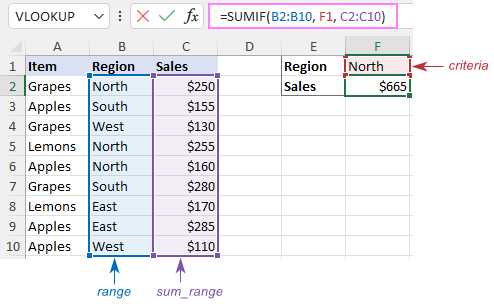
Note. The sum_range parameter actually defines only the upper leftmost cell of the range to be summed. The remaining area is defined by the dimensions of the range argument. In practice, this means that sum_range argument does not necessarily have to be of the same size as range argument, i. e. it may have a different number of rows and columns. However, the top left cell must always be the right one. For example, in the above formula, you can supply C2, or C2:C4, or even C2:C100 as the sum_range argument, and the result will still be correct. However, the best practice is to provide equally sized range and sum_range.
Note. The SUMIF function is case-insensitive by nature. However, it is possible to force it to recognize the text case. For full details, please see Case-sensitive SUMIF in Excel.
How to use SUMIF in Excel - formula examples
Hopefully, the above example has helped you gain some basic understanding of how the function works. Below you will find a few more formulas that demonstrate how to use SUMIF in Excel with various criteria.
SUMIF greater than or less than
To sum numbers greater than or less than a particular value, configure the SUMIF criteria with one of the following logical operators:
- Greater than (>)
- Greater than or equal to (>=)
- Less than (<)
- Less than or equal to (<=)
In the table below, supposing you wish to add up the sales numbers for the items that ship in 3 or more days. To express this condition, put a comparison operator (>) before the number and surround the construction in double quotes:
=SUMIF(C2:C10, ">3", B2:B10)
If the target number is in another cell, say F1, concatenate the logical operator and cell reference:
=SUMIF(C2:C10, ">"&F1, B2:B10)
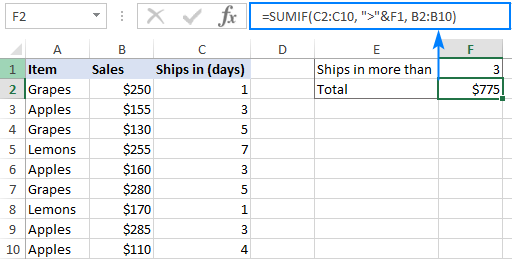
In a similar manner, you can sum values smaller than a given number. For this, use the less than (<) operator:
=SUMIF(C2:C10, "<3", B2:B10)
SUM IF equal to
A SUMIF formula with the "equal to" criteria works for both numbers and text. In such criteria, the equals sign is not actually required.
For instance, to find a total of the items that ship in 3 days, either of the below formulas will do:
=SUMIF(C2:C10, 3, B2:B10)
or
=SUMIF(C2:C10, "=3", B2:B10)
To sum if equal to cell, supply a cell reference for criteria:
=SUMIF(C2:C10, F1, B2:B10)
Where B2:B10 are the amounts, C2:C10 is the shipment duration, and F1 is the desired delivery time.
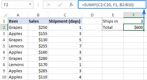
Likewise, you can use the "equal to" criteria with text values. For instance, to add up the Apples amounts, choose any of the formulas below:
=SUMIF(A2:A10, "apples", B2:B10)
=SUMIF(A2:A10, "=apples", B2:B10)
=SUMIF(A2:A10, F1, B2:B10)
Where A2:A10 is the list of items to compare against the value in F1.
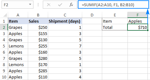
The above formulas imply that the criterion matches the entire cell contents. Consequently, the SUMIF function will add up Apples sales but not, say, Green Apples. To sum partial matches, construct the "if cell contains" criteria like in this SUMIF wildcard formula.
Note. Please pay attention that, in Excel SUMIF formulas, a comparison or equals operator should always be enclosed in double quotes, whether used on its own or together with a number or text.
SUM IF not equal to
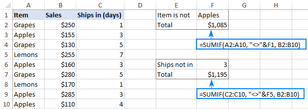
To build the "not equal to" criteria, use the "<>" logical operator.
When a value, either text or number, is hardcoded in the criteria, remember to surround the entire construction with double quotes.
For example, to sum the amounts with shipment other than 3 days, the formula goes as follows:
=SUMIF(C2:C10, "<>3", B2:B10)
To find a total of all the items except Apples, the formula is:
=SUMIF(A2:A10, "<>apples", B2:B10)
When the criterion is in another cell, concatenate the "not equal to" operator and a cell reference like this:
=SUMIF(A2:A10, "<>"&F1, B2:B10)
SUM IF blank
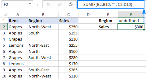
This example shows how to sum cells in one column if a corresponding cell in another column is blank. There are two formulas to fulfill the task. Which one to use depends on your interpretation of a "blank cell".
If "blank" means cells that contain absolutely nothing (no formula, no zero-length string returned by some other function), then use "=" for criteria. For example:
=SUMIF(B2:B10, "=", C2:D10)
If "blank" includes empty strings (for example, cells with a formula like =""), then use "" for criteria:
=SUMIF(B2:B10, "", C2:D10)
Both formulas return a total of sales for undefined regions, i.e. where a cell in column B is blank:
SUM IF not blank
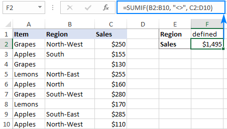
To make "if cell is not blank then sum" kind of formula, use "<>" as the criteria. This will add up all cells that contain anything in them, including zero-length strings.
For instance, here's how you can sum sales for all the regions, i.e. where column B is not blank:
=SUMIF(B2:B10, "<>", C2:D10)
Excel SUMIF with text criteria
When adding up numbers in one column based on text values in another column, it's important to differentiate between exact and partial match.
| Criteria | Formula Example | Description |
|---|---|---|
| Sum if equal to | Exact match: =SUMIF(A2:A8, "bananas", C2:C8) |
Sum values in cells C2:C8 if a cell in column A in the same row contains exactly the word "bananas" and no other words or characters. Cells containing "green bananas", "bananas green", or "bananas!" are not included. |
| Sum if cell contains | Partial match: =SUMIF(A2:A8, "*bananas*", C2:C8) |
Sum values in cells C2:C8 if a corresponding cell in column A contains the word "bananas", alone or in combination with any other words. Cells containing "green bananas", "bananas green", or "bananas!" are summed. |
| Sum if not equal to | Exact match: =SUMIF(A2:A8, "<>bananas", C2:C8) |
Sum values in cells C2:C8 if a cell in column A contains any value other than "bananas". If a cell contains "bananas" together with some other words or characters like "yellow bananas" or "bananas yellow", such cells are summed. |
| Sum if cell does not contain | Partial match: =SUMIF(A2:A8, "<>*bananas*", C2:C8) |
Sum values in cells C2:C8 if a cell in column A does not contain the word "bananas", alone or in combination with any other words. Cells containing "yellow bananas" or "bananas yellow" are not summed. |
For real-life formula examples, please check out Sum if equal to and Sum if not equal to.
In the next section, we'll take a closer look at SUMIF formulas with partial match.
SUMIF formulas with wildcard characters
To conditionally sum cells by partial match, include one of the following wildcard characters in your criteria:
- Question mark (?) to match any single character in a specific position.
- Asterisk (*) to match any number of characters.
Example 1. Sum values based on partial match
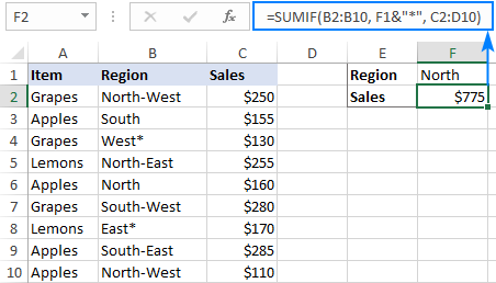
Suppose you wish to total sales for all northern regions, including North, North-East, and North-West. To have it done, put an asterisk right after the word "north":
=SUMIF(B2:B10, "north*", C2:D10)
An asterisk on both sides will also work:
=SUMIF(B2:B10, "*north*", C2:D10)
Alternatively, you can type the region of interest in a predefined cell (F1), and then concatenate a cell reference and a wildcard character enclosed in quotes:
=SUMIF(B2:B10, F1&"*", C2:D10)
Or
=SUMIF(B2:B10, "*"&F1&"*", C2:D10)
Example 2. Sum if cell contains * or ?
To match a literal question mark or asterisk, place a tilde (~) before the character, e.g. "~?" or "~*".
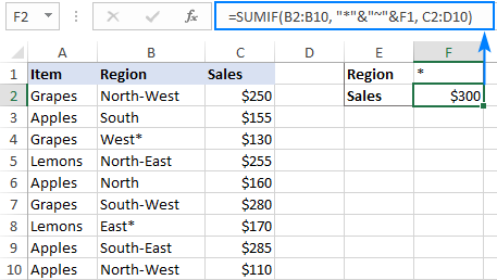
For example, to sum sales for the regions marked with *, use "*~*" for criteria. In this case, the first asterisk is a wildcard and the second one is a literal asterisk character:
=SUMIF(B2:B10, "*~*", C2:D10)
If the criteria (* in our case) is entered in a separate cell, then concatenate a tilde and the cell reference, like this:
=SUMIF(B2:B10, "*"&"~"&F1, C2:D10)
Example 3. Sum if another cell contains text
If your dataset contains various data types and you only want to sum cells corresponding to text values, the following SUMIF formulas will come in handy.
To add up values in cells C2:C8 if a cell in column A contains any text character(s):
=SUMIF(A2:A8,"?*", C2:C8)
To sum values in C2:C8 if a cell in column A contains any text value, including zero length strings:
=SUMIF(A2:A8,"*", C2:C8)
Both of the above formulas ignore non-text values such as numbers, dates, errors, and Booleans.
How to use Excel SUMIF with dates
Using dates as SUMIF criteria is very much like using numbers. The most important thing is to supply a date in the format that Excel understands. If you are not sure which date format is supported and which is not, the DATE function can be a solution.
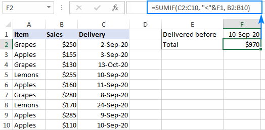
Assuming you are looking to sum sales for the items delivered before 10-Sep-2020, the criteria can be expressed in this way:
=SUMIF(C2:C10, "<9/10/2020", B2:B10)
or
=SUMIF(C2:C10, "<"&DATE(2020,9,10), B2:B10)
or
=SUMIF(C2:C10, "<"&F1, B2:B10)
Where F1 is the target date.
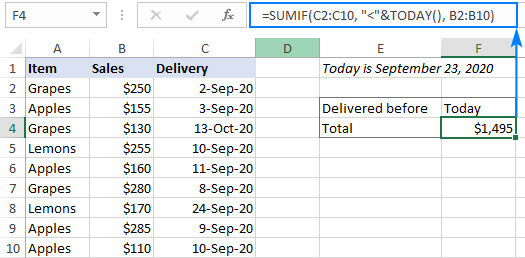
To sum cells based on today's date, include the TODAY function in your criteria. For example, that's how you calculate a total of sales with a delivery date prior to today:
=SUMIF(C2:C10, "<"&TODAY(), B2:B10)
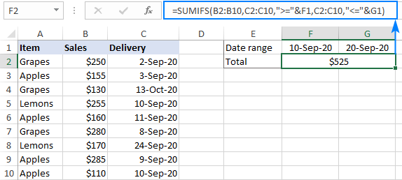
To sum within a date range, you need to define a smaller and larger date separately. This can be done with the help of the SUMIFS function that supports multiple criteria.
For example, to sum values in column B if a date in column C is between two dates, this is the formula to use:
=SUMIFS(B2:B10, C2:C10, ">="&F1, C2:C10, "<="&G1)
Where B2:B10 is the sum range, C2:C10 is the list of dates to check, F1 is the start date and G1 is the end date.
More formula examples can be found in SUMIFS with date range as criteria.
How to do SUMIF from another sheet
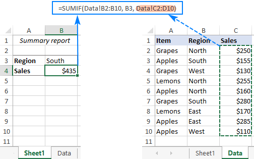
To conditionally sum data from a different sheet, provide external references for the SUMIF arguments. The easiest way is to start typing a formula, switch to another worksheet and select ranges using the mouse. Excel will insert all the references automatically, without you having to worry about the correct syntax.
For instance, the below formula will add up values in C2:C10 on the Data sheet based on the criteria in B3 on Sheet1:
=SUMIF(Data!B2:B10, B3, Data!C2:C10)
How to correctly use cell references in SUMIF criteria
To create a flexible formula, you normally insert all variable parameters in predefined cells instead of "hardcoding" them. With Excel SUMIF, that might be a bit of a challenge.
In the simplest case when summing "if equal to", you simply use a cell reference for criteria. For example:
=SUMIF(C2:C10, F1, B2:B10)
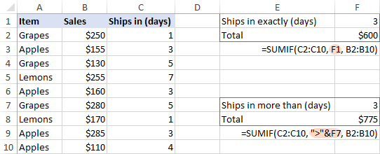
But when a cell reference is used together with a logical operator, the criteria should be provided in the form of a string. So, you use the double quotes ("") to start a text string and ampersand (&) to concatenate and finish the string off. For example:
=SUMIF(C2:C10, ">"&F7, B2:B10)
Please note that the comparison operators are enclosed in quotation marks while the cell references are not.
Why is my SUMIF formula not working?
There could be several reasons why Excel SUMIF is not working for you. Sometimes, your formula does not return what you expect only because the data type in a cell or in some argument isn't suited for the SUMIF function. Below is a list of important things to check.
1. SUMIF supports only one condition
The syntax of the SUMIF function has room for only one condition. To sum with multiple criteria, either use the SUMIFS function (adds up cells that meet all the conditions) or build a SUMIF formula with multiple OR criteria (sums cells that meet any of the conditions).
2. Range and sum_range should be of the same size
For a SUMIF formula to work correctly, the range and sum_range argument should have the same dimensions, otherwise you may get misleading results. The point is that Microsoft Excel does not rely on the user's ability to provide matching ranges, and to avoid possible inconsistency issues, it determines the sum range automatically in this way:
Sum_range defines only the upper left cell of the range that will be summed, the remaining area is determined by the size and shape of the range argument.
Given the above, the below formula will actually sum cells in C2:C10 and not in C2:D10. Why? Because range consists of 1 column and 9 rows, and so does sum_range.
=SUMIF(B2:B10, "north", C2:D10)
In older Excel versions, unequally sized ranges can cause lots of problems. In modern Excel, complex SUMIF formulas where sum_range has less rows and/or columns than range are also capricious. That is why it's a good practice to always define the same number of rows and columns for these two arguments.
3. Range and sum_range should be ranges, not arrays
Though SUMIF can process an array constant in criteria like shown in this example, it does not support arrays in range and sum_range. These two arguments can only be cell ranges.
5. SUMIF criteria syntax
For criteria, the SUMIF function allows using different data types including text, numbers, dates, cell references, logical operators (>, <, =, <>), wildcard characters (?, *, ~) and other functions. The syntax of such criteria is quite specific.
If the criteria argument includes a text value, wildcard character or logical operator followed by text, number or date, enclose the whole criteria in quotation marks. For example:
=SUMIF(B2:B10, "north*", C2:D10)
=SUMIF(C2:D10, ">100")
=SUMIF(B2:B10, "<>north", C2:D10)
=SUMIF(C2:C10, "<=9/10/2020", B2:B10)
When a logical operator is followed by a cell reference or another function, the criteria should be provided in the form of a string. So, you use an ampersand (&) to concatenate a logical operator and a reference or function. For example:
=SUMIF(B2:B10, ">"&F1)
=SUMIF(C2:D10, "<="&TODAY(), B2:B10)
4. SUMIF from another workbook not working
As with many Excel functions, SUMIF can refer to other sheets and workbooks, provided they are currently open.
For example, this formula will work fine as long as Book1 is open:
=SUMIF([Book1.xlsx]Sheet1!$A$2:$A$9,"apples",[Book1.xlsx]Sheet1!$F$2:$F$9)
And it will stop working as soon as Book1 is closed. This happens because the referenced ranges in closed workbooks get de-referenced into arrays. And since arrays are not supported in the range and sum_range arguments, SUMIF throws a #VALUE! error.
6. SUMIF does not recognize text case
By design, SUMIF in Excel is not case-sensitive, meaning it treats uppercase and lowercase letters as the same characters. To make a case-sensitive SUMIF formula, use the SUMPRODUCT function together with EXACT.
That's how to use SUMIF in Excel. Hopefully, our formula examples have given you some good insights. As always, I thank you for reading and hope to see you on our blog next week!
Practice workbook for download
Excel SUMIF examples (.xlsx file)
 by
by
343 comments
You are Great!
I have solved a problem that took a long time.
Thank you so much
Please, how can i find two cells having same numbers in excel. For example if A1 and B1 with numbers like A1=34 and B1=39. how can i find cells side by side with same value as 34,39. e.g H15=34,I15=39.
Thanks,
Jolly.O.A
I have 2 worksheets (1 is Contributions given - the other a Category Balance sheet). On the Contributions sheet I have Date, Name, Amount, Tithes, General Fund, Sunday School, etc. I will have multiple entries for each Date & I want to take the totals by Date & put on the Category Balance sheet. How can I create a formula that will look in the date column & total up each category based upon the date & autopopulate the results into the Category Balance sheet for each category?
How do you add cells in columnB. If B1 to B365 is equal to 1. If there is zero do not add and start again to the first row that is equal to 1. I need to know if there is straight 30, 60 and 90 days. Column A is the date field and Column B is the number of days without late, thus, contains either 1 (without late) or 0 (with late).
Ho many 30 days in a year. How many 60 days and how many 90 days without late?
I will appreciate any help.
Hi I am struggling with a cashflow and am hoping someone can help.
I have a cashflow laid out like this:
October 2016 November 2016 December 2016 January 2017 February 2017
£5000 £5000 £5000 £5000 £5000
I am trying to get a formula which automatically adjusts and counts the total of the cashflows from todays date to the end of my lease. Ie if todays date is November than count cash flows from November until end date.
Thanks
Like all other Excel Sum functions, SUMIF can only add up numbers, text values will be ignored. If there are some text-formatted digits in the column, you will have to convert them to numbers first, and you can find a handful of easy ways here: How to convert text-formatted digits to number in Excel.
Hi,
I have a table.
Name Subjects Marks
Amy Maths 58
Kishan Maths 78
Leon Maths 68
Ankit Maths 65
Rey Maths 53
Amy Science 57
Kishan Science 65
Leon Science 92
Ankit Science 39
Rey Science 98
Amy Social Science 69
Kishan Social Science 98
Leon Social Science 56
Ankit Social Science 87
Rey Social Science 96
Amy English 78
Kishan English 68
Leon English 54
Ankit English 63
Rey English 97
I have to copy same data in other table suing countifs. Can you please help me?
SL# Maths Science Social Science English
Amy
Kishan
Leon
Ankit
Rey
Average
how can I
my teacher told me to explain these formulars = sum(A2:F2)
Morning,
Probably simple but cannot get excel to do the following,
I want a cell to auto count when a single date is entered multiple times in a separate tab,
Ex - if 1/09/16 is entered 4 times then the cell in the other tab will count 4
if 2/09/2016 is entered 5 times then the cell in the other tab will count 5 and then if entered more times or deleted will auto adjust itself.
I want to sum a range of numbers based on a specific date -30 days. I am trying to sum up the hours flown in the past 30 days, 30 days, 90 days.
ex: 9/20/2016-30 days
9/20/2016-60 days
Hello need help for the following:
i have 2 collums, in collum A i have part no in collum B i have quantity.
Part numbers in collum A may be the same in more than one row.
So what i want to do is that.
find same part numbers in collum A, then sum their quantity from collum B and give me the total in collum c.
Something like that:
A B C
200855 10
200855 15
25
200856 25
200856 15
40
Thank you
I have table like below: how could I sum the cells that contain "S" in each column? help would be appreciated. in the below table the output should be .4 for column1 and .5 for column2
.5E .5E
.2U
.2G
.1S .2S
.1L .1L
.1U
.3S .3S
.7E .7E
Thanks Svetlana. You have really helped a great deal.
Please, how can i find two cells having same numbers in excel. For example if A1 and B1 with numbers like A1=34 and B1=39. how can i find cells side by side with same value as 34,39. e.g H15=34,I15=39.
Thanks,
Jolly.O.A
how to use sumif formula for datewise total for particular party and party's total for particular date in one coloumn
amt 3k if % less than 50%. to calculate total amt x 106%
amt 3k if % more than 50%. to calculate total amt x 115%
can advise on the formula?
Can anyone help me I have this 5000 list 1) column1- pan / name of customer
2)column various transaction types like P/T/S/R (as per the customer transaction details its short)
3) consists of total amounts and one customer has many transaction.. I used Sumif formula to get their total but I want a specific customer name showing total amount where as only transaction of (P)..
Please help
i need sumifs total for each person
A b c d e f
john 19,018 2,408 1,000 2,000 16,610 145,341
babu 4,563 578 1,000 2,000 3,985 15
raju 62,865 7,961 1,000 2,000 54,904 346,323
john 125,000 15,830 1,000 2,000 109,170 109,170
babu 63,697 8,066 1,000 2,000 55,631 55,631
raju 100,000 12,664 1,000 2,000 87,336 87,336
raju 50,806 6,434 1,000 2,000 44,372 1,352
raju 100,000 12,664 1,000 2,000 153 87,336
raju 59,115 7,486 1,000 5,000 132 51,629
babu 39,098 4,951 1,000 5,000 1,546 34,147
babu 500,000 63,319 1,000 5,000 15,463 436,681
babu 25,000 3,166 1,000 5,000 1,566 21,834
john 181,934 23,040 1,000 13,200 19,761 6,301
john 154,973 19,625 1,000 16,565 135,348 135,348
john 25,898 3,280 1,000 45,646 14,564 22,618
john 150,000 18,996 1,000 54,644 1,564 131,004
babu 612,971 12,019 1,000 5,465 68,546 600,952
babu 325,000 1,000 456,468 74,563 325,000
=SUMIF(A2:A10,"",C2:C10) sums values in column C if the corresponding cells in column A are not blank, i.e. they have some content. Therefore it will include values where the cell in A column contains a formula even if its result is "".
To work around this issue try =SUMIF(A2:A10,"><",C2:C10) instead.
i am using this =SUMIF(A3:A33,"<="&TODAY(),K3:K33) excel formula to calculate MTD whhich will compute sum upto today as i enter data everyday.
however need help to see how to calculate MTD average percentage !
[Note: column A being Date 1 to 31 and
column K being Occupancy%]
Thanks.
Please can one do nested If over 64 level of nexting?..
Kindly advise.
Thanks,
Jolly.O.A
Hi Jolly,
To my best knowledge, there is no way to nest more than 64 levels of If in Excel. You can check out the following alternatives to nested IF's. For example, you can use the CONCATENATE function that allows supplying up to 255 arguments in modern Excel versions, which equates to testing 255 different conditions.
BTW, did you get my email regarding the minus sign? In case it did not reach you for some reason, the problem was in your nested IF formula in cell B5. Because the numbers are enclosed in double quotes, Excel perceives them as text strings, and as the result other formulas referencing B5 yield wrong results. As soon as you remove the quotation marks, both formulas will work fine, and no minus sign will appear in B7.
IF A3 > B2 , SUBTRACT B2 FROM A3, AND IF B2 > A3 ,SUBTRACT A3 FROM B2. WITHOUT GETTING A MINUS(-) SIGN. BOTH CELL A3 AND B2 CONTAINS FORMULAS.
KINDLY ASSIST.
Hi Jolly,
Because you are always subtracting a smaller number from a larger number, there should be no minus sign in the result. It makes no difference whether the referenced cells are filled manually or using other formulas. It's difficult to say what is causing the minus sign to appear without seeing your worksheet. If you can send it to me (support@ablebits.com Att: Svetlana), I will try to help.
THANKS FOR THE SWIFT RESPONSE.
THE PROBLEM NOW IS THAT THE RESULT IS SHOWING A MINUS SIGN. MAYBE BECAUSE I ALREADY HAVE FORMULAS IN BOTH CELL A3 AND B2.HOW DO I CREATE THIS FORMULAR WITH GETTING A (-) SIGN. THANKS
This is exactly what I was looking for, thank you!!
help to make the formula to count total of following.
1 2 3 4 5 total
P P P H P ???
if p=1,than total sum=??
Hello,
Please help me with the formula/function to be used in order that i can get the total sum of the credit limit of a group of customers as shown below:
Customer Credit Orders
Cust#1 100 17
Cust#2 200 100
Cust#2 200 50
Cust#3 300 100
Cust#3 300 150
Cust#3 300 50
-------------------------
Total 600 467
=========================
Thanks a lot!
I am working on an monthly evaluation form for employees. It needs to sum cells and calculate a percentage but only if data is entered in a cell. An example of the basic set-up of the sheet is:
Professionalism: [Graded on a scale of 1 to 10]
Positive Attitude
Ability to relate to peers
Ability to relate to supers
Ability to relate to customers
Communicate orally
Communicate verbally
Support other beliefs
Respect differing opinions
Every employee would be graded each month and the scores would be averaged to give a percentage, but only if data is entered.
Jan Feb Mar Apr May Jun Jul Aug Sep Oct Nov Dec
5 6 7 60%
Thanks for helping me about the use of IF operator.
But I want to ask you how to use NOT operator within the AND and OR statement.
I have a Summary sheet full of all of the products which are available. It contains a Total number of products. The products are Booked In on one sheet and are then Booked Out from another, the Summary sheet contains a SUMIF-SUMIF which calculates the total. I require a warning system or conditional formatting to indicate the Min/Max for a total. Not all products have the same Min/Max.
The problem that I am having is that if I set up conditional formatting for specific cells and a new product is added, it moves the conditional formatting to another cell. In theory is it possible to make sure the conditional formatting sticks with its specific cell/product number? Or is there another method?
Can someone PLEASE help me?
I am trying to get a some of column A1:A1500 (only numerbic values) however, I have 2 additional conditions - I only want Excel to add the numerbic values in A1:A1500 for Nike's (type of sneakers) and the color Pink (color)
F:F is where the different types of Sneakers are listed and and column H:H is the various colors. I am trying to create a formula that will add (total sum) of the #'s of sneakers bought per customer (0-17) which is in column A:A - Pink Nike's ONLY?
Thanks in advance!
Hello,
I need to use a SUMIF formula I am pretty sure.
I have one sheet with outstanding invoices on it, and another sheet with a total for each customer as they aid I mark them YES for paid.
I need to work out what the formula can be so the paid invoices are not included in the total for outstanding.
Can anyone help?
Hi,
I want to use special character as >, 1 5
>1 10
|K 3
|K 1
Summary
Codes Amount
>1 15
|K 4
I need to use sumifs because i had multiple conditions in my table
Thank
Hi my homework says "In cell B33, enter a formula to add the individual 5 cells one at a time." how do I go about doing that?
Hi, I just happen to be on the site to see if there was an answer to my question.
For you, the easiest way is just to click on B33, enter =SUM(B1:B5) into the formula space, click the check mark next to the fx icon.
If you did it correctly then when you enter the values in cells B1 through B5 then B33 will add those independent values.
First Example:
A1 (Date); B1 (Bucket Size of 2.5 gallons); C1(Seconds To Fill Bucket); D1 (Gallons Per Minute).
Quest:
A1 (Date); B1 (Seconds To Fill Bucket);C1
Gallons Per Minute
Hi,
I’m cyber (computer) un-savvy . . .
I succeeded with three cells, in that, that equation =SUM(B1/C1*60) imposed in D1 will provide me with a correct answer. . Note, A1 is just the date of occurrence and is NOT necessary for the equation.
My quest is to formulate the equation so that it only involves two cells. B1 represents the constant (2.5 gallon bucket) that is divided by a variable (time of seconds to fill the bucket) that is entered into the cell, and C1 is the hiddeb equation that displays the answer (gpm). In essence, the equation is 2.5/B1*60=gpm . . . 2.5 is a constant bucket size, B1 is the variable of time (seconds to fill the bucket), *60 is a constant (60 seconds) = ANSWER (gallons per minute)
I have partial success, in that, C1’s equation =SUM(2.5/A1*60) functions if A1’s value is less or greater than 0 (zero). However, with the aforementioned equation, if the B1 value is 0 (zero) or left empty (implication that a sample was not obtained for that date) then there is an annoying and always present cell admonition of #DIV/0!.
Can you help???
Blessings,
Tim
I have never commented on such a forum before. However, thought you deserved truck loads of positive feedback on a concise, easy to understand, educational post. Thank you.
I wish to set up a criteria in such a way that it adds numbers in a range but the criteria excludes certains conditions within the criteria range.
Row A B
1 212200 10
2 218000 20
3 214000 40
4 215000 50
5 216000 60
6 217000 80
I this example I want to add up column b(b1:b6), criteria range (A1:A6), criteria is anything => 212200, but <=217000 and exclude 215000 to 216000.
Please help...
Hello, I cam trying to create a formula where I have 2 cells - one is the gross weight and the other is the dimensional weight. sometimes it differs on which one is greater. I need to create a sum of multiplying the charge by which ever the weights is greater. Can you please help me?
I am trying to work on a sheet where i have customer sales details of two products from which i want to calculate which customer has purchased what product in total. for one i cn calculate using "sumif" formula but its difficult to change the for formula for each customer.. can you please suggest me
hi
i have row with the following data in the cells:
A3=20, B3=50, C3=PAID, D3=60, E3=PAID, F3=60, G3=PAID, H3=20, I3=40, J3=60
I WANT TO SUM THE FOLLOWING CELLS: A3, C3, E3, F3, J3
AS A RESULT I GET AN ERROR NAMED "VALUE".
HOW CAN I SUM THESE CELLS WITHOUT GETTING AN ERROR.
THANK YOU,
ZVI
Hi
I am needing a formula that sums only if both cells have a value.
And that answer will be multiplied by another cell
For example =a25+b25*g28
The formula is put into c28, I don't want anything appearing in c28 until both a25 and b25 contain a number or value, It needs to wait to add until I put a number into both cells,
Thank you soo much for your time,
I am useing 2013 excel
Hi
I'm trying to set up a prepayments schedule and I have the start date, end date, amount and daily rate shown is separate cells for an invoice. I have 12 further columns for each month of the year. I would like to have the invoice amount split between the months according to the number of days relevant to the month. eg an invoice may run from 13th of 1 month to the 12 of another. is there a formula that will calculate the number of days relevant for the month and multiply this by the daily rate?
I am trying to create a formula that puts in a cell an invoice amount based on different date ranges.
The invoice amount will be $1000 if the invoice date is between 2 date ranges in a month say August (100 %)
The invoice amount will then drop to 900 if between 2 date ranges in September(90%)
The invoice amount drops to say $800 if between 2 date ranges in October.
Hello Michael,
You can use the following kind of formula for your task:
=IF(AND(A1>DATE(2015,8,1), A1<DATE(2015,8,31)),1000,IF(AND(A1>DATE(2015,9,1), A1<DATE(2015,9,30)),900,IF(AND(A1>DATE(2015,10,1), A1<DATE(2015,10,31)),800, 1000)))
It allows you to list several conditions for different values that you want to show. Please also see for examples of using dates in your formulas.
I don't think this site is being monitored anymore. I don't see any answers.
Hello?
Hello Jeannie,
We apologize for the delay, it takes time to look at all the comments we get and provide a solution. Please find the formula for your task above.
Hello,
Column A i have date starting from 1 to 30 up to rows 30...
Column B i have Day from Monday to Saturday up to rows 30...
Column C i have Traget hours from 16 to 50 hours with if logic function base on value of column F ( Total of column D and E )
Now i want to apply sumif formula at the end for day for Example if the day is Friday then ...
=SUMIF(A1:A30,"Friday",B1:B30 )
But formula not given any error or and doinn sum also..
But same formula when I apply in column those have direct value ( not coming from if fuction ) it's working properly.
Thanks if anyone can give anwser
Hello Hari Mohan,
As you have dates in column A, days in column B, and the hours to sum in column C, your formula should have columns B and C as the range and sum range instead of columns A and B, i.e.:
=SUMIF(B1:B30,"Friday",C1:C30)
Hello,
Can you help me regarding sumif formula which not working properly.
Name of DAy form Sunday to Saturday in Column A and number of working hours in column B ( and column B all values are base on IF formula ).
When I want to apply SUMIF formula its not working because my target hours base on if formula in column B.
Same formula when I apply in a simple way then its working properly.
Your help with my problem would be appreciated.
It is probably a simple code, but I'm struggling with it.
Every 4 years I have to calculate how many precinct committee people a precinct can have at each site.
For less than 1,000 voters, it is 1 pair
For more than 1,001 voters, it is 2 pair
For more than 2001 voters, it is 3 pair
The form is a 3 columns: first column is the name of the precinct, 2nd column is the total voters and 3rd column shows how many precinct committee people is allowed.
Precinct Name Total Reg Voters Allowable Pairs
Sumter Place Rec Room 3432
Can you help?
Since I have not heard back on my question, I can only assume
that there isn't a formula?
Jeannie
Hello Jeannie,
I'm really sorry that you had to wait for the formula.
You can use the IF function with a combination of your conditions for your task:
=IF(B2<1001,1, IF(B2<2001, 2, 3))
You need to enter this formula into column C and copy it across the column.
Here B2 is the cell with the "total reg voters". If there are fewer than 1001, the formula will show 1, if there are fewer than 2001, it will show 2, otherwise it will show 3.
OK. My prior post somehow did not come across what I had written. Trying again
Create a formula with sumif(s) using >0 or <0 in the equation. Keeps returning either a "false", or sum of entire range.
sum range = BSJun_Act
criteria = BSMap_to,"Interco"
Hello Diana,
It sounds like you need to use the SUMIFS function that lets you specify several conditions. E.g.
=SUMIFS(B15:B27,A15:A27,"Interco",B15:B27,">0")
The range A15:A27 is checked for the word "Interco", B15:B27 is checked for the condition ">0".
You can use named ranges instead of the range references by spelling them this way:
=SUMIFS(BSJun_Act,BSMap_to,"Interco",BSJun_Act,">0")
If you get an error, please make sure both ranges are of the same size.
I am trying to create a sumif of sumifs formula using named ranges and using either a >0 or 0",SUMIF(BSMap_to,"Interco",BSJun_Act)0)
IF(Sumif(BSMap_to,"Interco")>0,SUMIF(BSMap_to,"Interco",BSJun_Act))
It seems to work if I use an actual range like A15:A27, but I can't seem to find the answer to get this formula to work using named ranges where the range is not in a series.
Thanks for your help!
Hi, Svetlana,
I am kind of trying to right down a formula that would count me the following condition:
- if the certain cells sum (lets say B2 to Q2) would be more or equal to 80, then the sums of the cells B2:B3 should be multiplied by 2 and to it cells B4 and B5 should be added, if the cells sum (B2 to Q2) would be more or equal to 160, then the sums of the cells B2:B3 should be multiplied by 3 and to it cells B4 and B5 should be added, if neither are correct (that is the value of the cells sum is less than 80) then the formula should return value D5.
Even better formula would be:
- when the sum of the cells reaches number 80, then the sum of the cells B2:B3 should be multiplies by 2 and to it cells B4 and B5 added, when reaches 160 - multiplied by 3 and to it cells B4 and B5 added. If the sum is less then 80, then the value should be D5.
I can't get correct formula anyhow...
Would really appreciate Your insights on this one. Thanks in advance.
Hello Justin,
You can use the following formula for your task:
=IF(SUM(B2:Q2)>160,SUM($B$2:$B$3)*3+SUM($B$4:$B$5),IF(SUM(B2:Q2)>80,SUM($B$2:$B$3)*2+SUM($B$4:$B$5),D5))
If you'd like the summed ranges to shift as you copy the formula, please make the references relative, i.e.:
=IF(SUM(B2:Q2)>160,SUM(B2:B3)*3+SUM(B4:B5),IF(SUM(B2:Q2)>80,SUM(B2:B3)*2+SUM(B4:B5),D5))
How to sort data when cell are merged and wraped
Hello,
You can sort merged cells only if they are of the same size: select them and click the Sort icon.
Otherwise you need to unmerge all cells in the range before sorting.