The tutorial shows how to build an amortization schedule in Excel to detail periodic payments on an amortizing loan or mortgage.
An amortizing loan is just a fancy way to define a loan that is paid back in installments throughout the entire term of the loan.
Basically, all loans are amortizing in one way or another. For example, a fully amortizing loan for 24 months will have 24 equal monthly payments. Each payment applies some amount towards principal and some towards interest. To detail each payment on a loan, you can build a loan amortization schedule.
An amortization schedule is a table that lists periodic payments on a loan or mortgage over time, breaks down each payment into principal and interest, and shows the remaining balance after each payment.
How to create a loan amortization schedule in Excel
To build a loan or mortgage amortization schedule in Excel, we will need to use the following functions:
- PMT function - calculates the total amount of a periodic payment. This amount stays constant for the entire duration of the loan.
- PPMT function - gets the principal part of each payment that goes toward the loan principal, i.e. the amount you borrowed. This amount increases for subsequent payments.
- IPMT function - finds the interest part of each payment that goes toward interest. This amount decreases with each payment.
Now, let's go through the process step-by-step.
1. Set up the amortization table
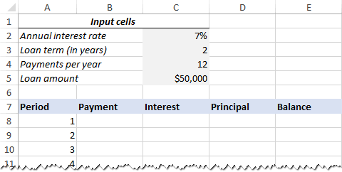
For starters, define the input cells where you will enter the known components of a loan:
- C2 - annual interest rate
- C3 - loan term in years
- C4 - number of payments per year
- C5 - loan amount
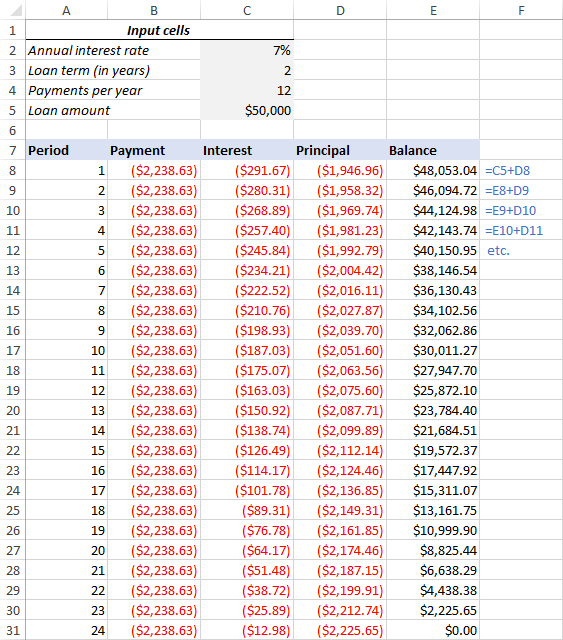
The next thing you do is to create an amortization table with the labels (Period, Payment, Interest, Principal, Balance) in A7:E7. In the Period column, enter a series of numbers equal to the total number of payments (1- 24 in this example):
With all the known components in place, let's get to the most interesting part - loan amortization formulas.
2. Calculate total payment amount (PMT formula)
The payment amount is calculated with the PMT(rate, nper, pv, [fv], [type]) function.
To handle different payment frequencies correctly (such as weekly, monthly, quarterly, etc.), you should be consistent with the values supplied for the rate and nper arguments:
- Rate - divide the annual interest rate by the number of payment periods per year ($C$2/$C$4).
- Nper - multiply the number of years by the number of payment periods per year ($C$3*$C$4).
- For the pv argument, enter the loan amount ($C$5).
- The fv and type arguments can be omitted since their default values work just fine for us (balance after the last payment is supposed to be 0; payments are made at the end of each period).
Putting the above arguments together, we get this formula:
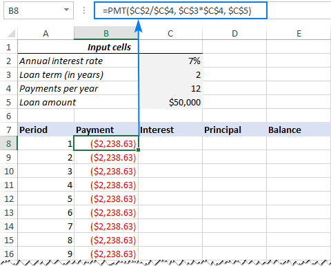
=PMT($C$2/$C$4, $C$3*$C$4, $C$5)
Please pay attention, that we use absolute cell references because this formula should copy to the below cells without any changes.
Enter the PMT formula in B8, drag it down the column, and you will see a constant payment amount for all the periods:
3. Calculate interest (IPMT formula)
To find the interest part of each periodic payment, use the IPMT(rate, per, nper, pv, [fv], [type]) function:
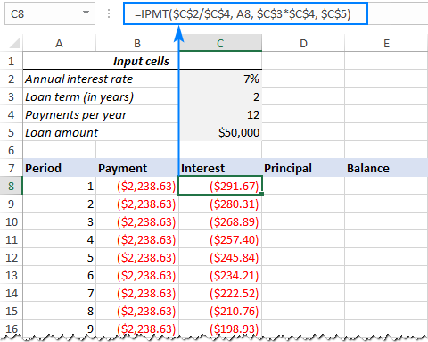
=IPMT($C$2/$C$4, A8, $C$3*$C$4, $C$5)
All the arguments are the same as in the PMT formula, except the per argument that specifies the payment period. This argument is supplied as a relative cell reference (A8) because it is supposed to change based on the relative position of a row to which the formula is copied.
This formula goes to C8, and then you copy it down to as many cells as needed:
4. Find principal (PPMT formula)
To calculate the principal part of each periodic payment, use this PPMT formula:
=PPMT($C$2/$C$4, A8, $C$3*$C$4, $C$5)
The syntax and arguments are exactly the same as in the IPMT formula discussed above:
This formula goes to column D, beginning in D8:
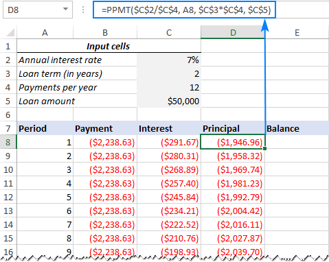
Tip. To check whether your calculations are correct at this point, add up the numbers in the Principal and Interest columns. The sum should be equal to the value in the Payment column in the same row.
5. Get the remaining balance
To calculate the remaining balance for each period, we'll be using two different formulas.
To find the balance after the first payment in E8, add up the loan amount (C5) and the principal of the first period (D8):
=C5+D8
Because the loan amount is a positive number and principal is a negative number, the latter is actually subtracted from the former.
For the second and all succeeding periods, add up the previous balance and this period's principal:
=E8+D9
The above formula goes to E9, and then you copy it down the column. Due to the use of relative cell references, the formula adjusts correctly for each row.
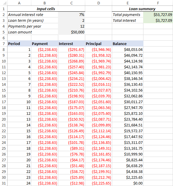
That's it! Our monthly loan amortization schedule is done:
Tip: Return payments as positive numbers
Because a loan is paid out of your bank account, Excel functions return the payment, interest and principal as negative numbers. By default, these values are highlighted in red and enclosed in parentheses as you can see in the image above.
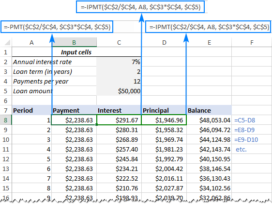
If you prefer to have all the results as positive numbers, put a minus sign before the PMT, IPMT and PPMT functions.
For the Balance formulas, use subtraction instead of addition like shown in the screenshot below:
Amortization schedule for a variable number of periods
In the above example, we built a loan amortization schedule for the predefined number of payment periods. This quick one-time solution works well for a specific loan or mortgage.
If you are looking to create a reusable amortization schedule with a variable number of periods, you will have to take a more comprehensive approach described below.
1. Input the maximum number of periods
In the Period column, insert the maximum number of payments you are going to allow for any loan, say, from 1 to 360. You can leverage Excel's AutoFill feature to enter a series of numbers faster.
2. Use IF statements in amortization formulas
Because you now have many excessive period numbers, you have to somehow limit the calculations to the actual number of payments for a particular loan. This can be done by wrapping each formula into an IF statement. The logical test of the IF statement checks if the period number in the current row is less than or equal to the total number of payments. If the logical test is TRUE, the corresponding function is calculated; if FALSE, an empty string is returned.
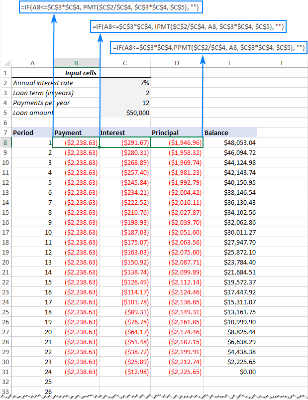
Assuming Period 1 is in row 8, enter the following formulas in the corresponding cells, and then copy them across the entire table.
Payment (B8):
=IF(A8<=$C$3*$C$4, PMT($C$2/$C$4, $C$3*$C$4, $C$5), "")
Interest (C8):
=IF(A8<=$C$3*$C$4, IPMT($C$2/$C$4, A8, $C$3*$C$4, $C$5), "")
Principal (D8):
=IF(A8<=$C$3*$C$4,PPMT($C$2/$C$4, A8, $C$3*$C$4, $C$5), "")
Balance:
For Period 1 (E8), the formula is the same as in the previous example:
=C5+D8
For Period 2 (E9) and all subsequent periods, the formula takes this shape:
=IF(A9<=$C$3*$C$4, E8+D9, "")
As the result, you have a correctly calculated amortization schedule and a bunch of empty rows with the period numbers after the loan is paid off.
3. Hide extra periods numbers
If you can live with a bunch of superfluous period numbers displayed after the last payment, you can consider the work done and skip this step. If you strive for perfection, then hide all unused periods by making a conditional formatting rule that sets the font color to white for any rows after the last payment is made.
For this, select all the data rows if your amortization table (A8:E367 in our case) and click Home tab > Conditional formatting > New Rule… > Use a formula to determine which cells to format.
In the corresponding box, enter the below formula that checks if the period number in column A is greater than the total number of payments:
=$A8>$C$3*$C$4
Important note! For the conditional formatting formula to work correctly, be sure to use absolute cell references for the Loan term and Payments per year cells that you multiply ($C$3*$C$4). The product is compared with the Period 1 cell, for which you use a mixed cell reference - absolute column and relative row ($A8).
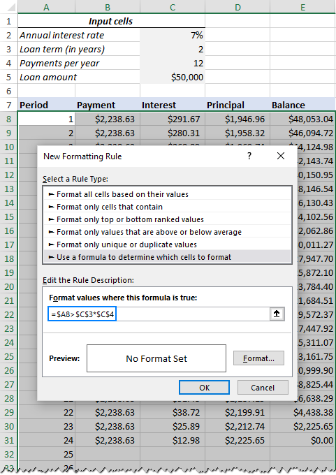
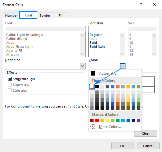
After that, click the Format… button and pick the white font color. Done!
4. Make a loan summary
To view the summary information about your loan at a glance, add a couple more formulas at the top of your amortization schedule.
Total payments (F2):
=-SUM(B8:B367)
Total interest (F3):
=-SUM(C8:C367)
If you have payments as positive numbers, remove the minus sign from the above formulas.
That's it! Our loan amortization schedule is completed and good to go!
How to make a loan amortization schedule with extra payments in Excel
The amortization schedules discussed in the previous examples are easy to create and follow (hopefully :). However, they leave out a useful feature that many loan payers are interested in - additional payments to pay off a loan faster. In this example, we will look at how to create a loan amortization schedule with extra payments.
1. Define input cells
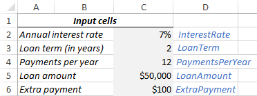
As usual, begin with setting up the input cells. In this case, let's name these cells like written below to make our formulas easier to read:
- InterestRate - C2 (annual interest rate)
- LoanTerm - C3 (loan term in years)
- PaymentsPerYear - C4 (number of payments per year)
- LoanAmount - C5 (total loan amount)
- ExtraPayment - C6 (extra payment per period)
2. Calculate a scheduled payment
Apart from the input cells, one more predefined cell is required for our further calculations - the scheduled payment amount, i.e. the amount to be paid on a loan if no extra payments are made. This amount is calculated with the following formula:
=IFERROR(-PMT(InterestRate/PaymentsPerYear, LoanTerm*PaymentsPerYear, LoanAmount), "")
Please pay attention that we put a minus sign before the PMT function to have the result as a positive number. To prevent errors in case some of the input cells are empty, we enclose the PMT formula within the IFERROR function.
Enter this formula in some cell (G2 in our case) and name that cell ScheduledPayment.

3. Set up the amortization table
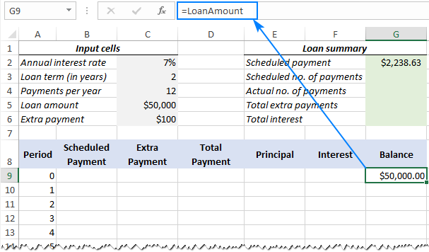
Create a loan amortization table with the headers shown in the screenshot below. In the Period column enter a series of numbers beginning with zero (you can hide the Period 0 row later if needed).
If you aim to create a reusable amortization schedule, enter the maximum possible number of payment periods (0 to 360 in this example).
For Period 0 (row 9 in our case), pull the Balance value, which is equal to the original loan amount. All other cells in this row will remain empty:
Formula in G9:
=LoanAmount
4. Build formulas for amortization schedule with extra payments
This is a key part of our work. Because Excel's built-in functions do not provide for additional payments, we will have to do all the math on our own.
Note. In this example, Period 0 is in row 9 and Period 1 is in row 10. If your amortization table begins in a different row, please be sure to adjust the cell references accordingly.
Enter the following formulas in row 10 (Period 1), and then copy them down for all of the remaining periods.
Scheduled Payment (B10):
If the ScheduledPayment amount (named cell G2) is less than or equal to the remaining balance (G9), use the scheduled payment. Otherwise, add the remaining balance and the interest for the previous month.
=IFERROR(IF(ScheduledPayment<=G9, ScheduledPayment, G9+G9*InterestRate/PaymentsPerYear), "")
As an extra precaution, we wrap this and all subsequent formulas in the IFERROR function. This will prevent a bunch of various errors if some of the input cells are empty or contain invalid values.
Extra Payment (C10):
Use an IF formula with the following logic:
If the ExtraPayment amount (named cell C6) is less than the difference between the remaining balance and this period's principal (G9-E10), return ExtraPayment; otherwise use the difference.
=IFERROR(IF(ExtraPayment<G9-E10, ExtraPayment, G9-E10), "")
Tip. If you have variable additional payments, just type the individual amounts directly in the Extra Payment column.
Total Payment (D10)
Simply, add the scheduled payment (B10) and the extra payment (C10) for the current period:
=IFERROR(B10+C10, "")
Principal (E10)
If the schedule payment for a given period is greater than zero, return a smaller of the two values: scheduled payment minus interest (B10-F10) or the remaining balance (G9); otherwise return zero.
=IFERROR(IF(B10>0, MIN(B10-F10, G9), 0), "")
Please note that the principal only includes the part of the scheduled payment (not the extra payment!) that goes toward the loan principal.
Interest (F10)
If the schedule payment for a given period is greater than zero, divide the annual interest rate (named cell C2) by the number of payments per year (named cell C4) and multiply the result by the balance remaining after the previous period; otherwise, return 0.
=IFERROR(IF(B10>0, InterestRate/PaymentsPerYear*G9, 0), "")
Balance (G10)
If the remaining balance (G9) is greater than zero, subtract the principal portion of the payment (E10) and the extra payment (C10) from the balance remaining after the previous period (G9); otherwise return 0.
=IFERROR(IF(G9 >0, G9-E10-C10, 0), "")
Note. Because some of the formulas cross reference each other (not circular reference!), they may display wrong results in the process. So, please do not start troubleshooting until you enter the very last formula in your amortization table.
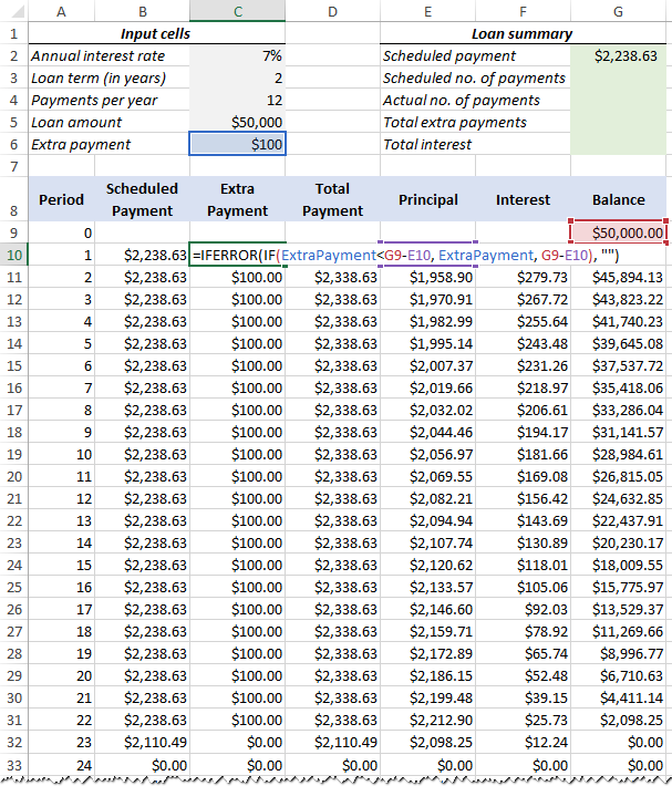
If all done correctly, your loan amortization schedule at this point should look something like this:
5. Hide extra periods
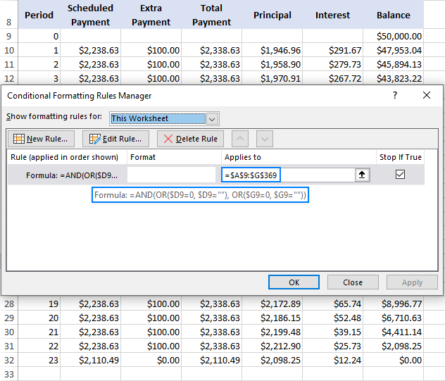
Set up a conditional formatting rule to hide the values in unused periods as explained in this tip. The difference is that this time we apply the white font color to the rows in which Total Payment (column D) and Balance (column G) are equal to zero or empty:
=AND(OR($D9=0, $D9=""), OR($G9=0, $G9=""))
Voilà, all rows with zero values are hidden from view:
6. Make a loan summary
As a finishing touch of perfection, you can output the most important information about a loan by using these formulas:
Scheduled number of payments:
Multiply the number of years by the number of payments per year:
=LoanTerm*PaymentsPerYear
Actual number of payments:
Count cells in the Total Payment column that are greater than zero, beginning with Period 1:
=COUNTIF(D10:D369,">"&0)
Total extra payments:
Add up cells in the Extra Payment column, beginning with Period 1:
=SUM(C10:C369)
Total interest:
Add up cells in the Interest column, beginning with Period 1:
=SUM(F10:F369)
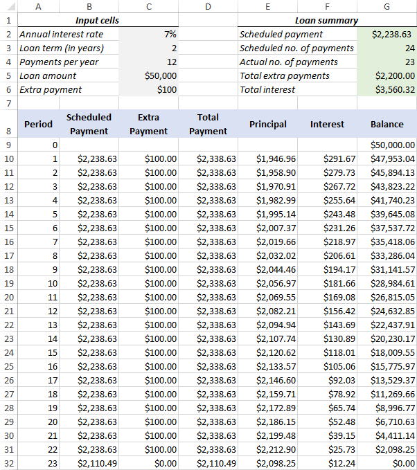
Optionally, hide the Period 0 row, and your loan amortization schedule with additional payments is done! The screenshot below shows the final result:
Amortization schedule Excel template
To make a top-notch loan amortization schedule in no time, make use of Excel's inbuilt templates. Just go to File > New, type "amortization schedule" in the search box and pick the template you like, for example, this one with extra payments:
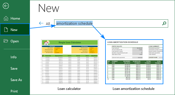
Then save the newly created workbook as an Excel template and reuse whenever you want.
That's how you create a loan or mortgage amortization schedule in Excel. I thank you for reading and hope to see you on our blog next week!
Available downloads
Amortization Schedule examples (.xlsx file)
 by
by
88 comments
To the author, great table!. I was looking for something like this. I would like to change something on it though and not to sure of the process. I notice when filling in the loan term the cells automatically populate which is brilliant! However, when putting in 25 or 30 years the max cells that populate end at cell 369. How would I change that to match 25 years? I've tried auto filling the other cells but they stay blank.
This is a great tool. My target is to dynamically revisit my current Mortgage Balance with large payments (e.g., $100,000.00 at a time to see what the imapcaat would be on the payment. The concept is to pay the current Mortgage amount offr Early.
Thanks....
Jim Kerr, Sr.
Hi,
Good day. Thanks for the wonderful amortization tool and the steps tutorial.
Have you done one with a principle moratorium option? Will appreciate receiving a copy of the same via mail.
Thanks.
Bosco
Thank you for the tutorial on making an Amortization Schedule. I learned a few things from you as well.
Awesome! Great help! Thank you.
Am I the only one that is lost here? When setting up the table for extra payments, when i copy the formulas down for the amortization table the boxes the formula references count up as well and start referencing incorrect numbers and in some cases words. How do i copy the formula down the chart but still reference the correct boxes at the top of the table?
Notice how some earlier formulas use $ symbols, such as $C$4. This locks the formula on only ever use the data in C4. Without that, then when you auto fill the formula, it changes itself to C5, C6, C7, etc.
There are some important uses for the shifting cell reference, such as when calculating remaining balance. You want it to use the formula from the previous row, and you want that to keep shifting as it goes down.
Very helpful, thank you very much for this tutorial.
How can I generate this in excel?
A loan of 180,000,000.00 at 22%. Tenor: 48 months(inclusive of 6 months moratorium). The payment plan is 14 quarterly repayment of principal of 12.857 million while interest will be serviced monthly throughout the duration of the facility. Penal rate for late payment is 1% flat on unpaid instalment in addition to the current interest repayment of rate applied on the outstanding amount.
Hi Everyone,
How do i claculate the monthly scheduled payment for a loan with a tenure of 5 years and a grace period granted for the repayment for the 1st nine months of the Year 1.
Appreciate your kind response.
Do you know of a single amortization template where you can add new loans after the first loan started amortizing and have a combined worksheet with the blended information?
i.e. Loan1 $10,000, 6%, Start Date 01/01/21, term 60 months and Loan2 $12,000, 5%, Start Date 03/01/21, term 72 months.
I know there are bank software package for this, but am trying to do it in Excel.
Thanks,
If you calculate monthly payments and then pay bi-weekly. How do you account for early payment and extra payment? Eg if your payment is 1200, and in month 1 you pay 1200. Let’s say 400 goes towards principal and 800 to interest, on day 30 your principal goes down 400, but, if you are paid bi-weekly and pay 600 at day 14 (200 principal and 400 interest) and 600 on day 28 you will make an extra payment in the year, and the 200 decrease on day 14 decreases the balance for interest on day 28. How do you account for this?
tnx. Good prt
tnx.
Greetings,
Thank you for sharing this tutorial. I'm wondering if it would be possible to get the information in the Loan Summary section without building an amortization schedule? I want a simple clean sheet to compare payment options. I know I can build the amortization schedules on a different sheets and reference those fields on a new sheet, but I have a lot of different options to consider, and would prefer not to build amortizations schedules for each if it's possible. Thanks.
Well articulated. Good presentation.
I believe there is an error in your loan summary calculations. Although the 30 year loan example has 360 monthly payments, with the FINAL payment in row 367 (because the first 8 rows are header). In other words, you show total payments (F2): =-SUM(B8:B360), but shouldn't it be payments (F2)=-SUM(B8:B367)? And instead of total interest (F3):=-SUM(C8:C360), shouldn't it be total interest (F3):=-SUM(C8:C367)? Also, any chance you could tell me how to modify the spreadsheet for a loan that is interest-only for the first 10 years, then typical Principal & Interest amortization for the final 20 years?
Oops there was an error in my note about the error LOL! I meant to say "Although the 30-year loan example has 360 monthly payments, with the FINAL payment in row 367 (because the first SEVEN rows are header), the totals formulas in F2 and F3 only include up to row 360)". Thanks again. Any help on a loan with interest-only in the beginning, then switching to typical amortization at some point, would be much appreciated.
Hi Beth,
Oops, you are absolutely right. Fixed, thank you!
Hi can someone help... if I am paying for the principle + interest only for the 7th to the 12 month, and 1st to 6 th month will be interest only, so how do i put this in the excel.
Thanks :-)
Sangita
Thanks for this, I've tried both your template and Microsoft's one to extend beyond 360months. How can I fix this to allow me spread payments to 35years for example?
Ignore my message, I've just used your tutorial to build from scratch. Thanks.
How to modify the interest rate changes, frequently? please reply
How about the short term?? I mean loan term is under 1 year (8 months), can I use this formula as well?
This table is very helpful. However how can I create amortization table that shows the monthly payments of the APR compounding daily, monthly, and annually
Hi Svetlana,
Thankyou for building this spreadsheet, it's very helpful. I was wondering how I could include a monthly fee into the calculations?
Regards
David
One easy way would be to add it to the Remaining Balance column. In A7 type "Monthly Fee" and then in C7 type in the amount of the fee. For example, if the fee is $25, then type "25" into C7.
Next, add $C$7 to the Balance column.
Doing that will also increase the number of payments. For example, a 30 year mortgage will not be paid off in 30 years with extra fees being thrown onto it, UNLESS those fees are also automatically included in the payment amount. It may be wise to add $C$7 to the Payment column, too.
HI,
Please can you tell me how I would create an amortization schedule, where there are delayed payments for the first 6 months of a five year term.
Thanks so much.
how do I add grace period? I am getting a loan for 15 years, but I am not paying anything during initial 2 years. How shall I calculate that? another thing is that my annual interest rate is different during the grace period and remaining period. I just cannot put these two parameters in the amortization shcedule
Hi Team,
I need your assistance to calculate 20% fortnightly and spread over a number of repayments.
Say, K1000 is loan out to customers with an interest rate of 20% including a processing fee of 2% on the loan amount. How much can be repaid over 5 fortnights or up to 16 fortnight (8 months).
No. of repayments in fortnights
Amount (Kina) 5 6 7 8 9 10 11 12 13 14 15 16 17
500
600
700
1000
1500
2000
Amount will increase
Kindly work on my request and advise me
Thank you,
Inara 7086 1814
A loan was made with the following factors $17000, 2.0%, payment of $200 Monthly. Approx time 8 years. Unfortunately, the payments are sometimes over and sometimes Zero. When I use the summary for extra payment that you provided, it calculates the over payments, but with a $0.00 payment, it just leaves it as the previous months balance. Should there not be added interest for the missed payment?
Thank you.
Thank you so much! Your tutorial was easy to follow for me.
Thank you for the great write-up
How do i calculate interest on a loan with moratorium period for first few months? How would the amortization for such a loan be?
THE TABLE IS WONDERFUL
Can you add the following:
start date of loan
Due Date of payment
Also ion the extra payment can you add the facility where in the person repays the loan with varied payments, like in your example your schedules payment is 2238.63, now if the persons pays 5000 in any month then the tenure should reduce however instead of the 2238.63 he pays nothing or less then there should be a additional charge of the interest lost by extending the tenure. Is that possible
Hello, what if the bank charges a yearly service fee of $500. How do I incorporate this into the spreadsheet?
Hi Svetlana,
Thank you soooooo much! I've spent many hours looking for a way to calculate balance owed with varying extra payments and there is nothing else out there! Very Nice! Very Professional! You are the best!
Please i need a loan amortization excel sheet that has biweekly repayment. and loan terms. 3 months, 6 months, 10 months,
appreciate your effort
How do I insert a differnet %rate without changing the existing data? We went from a 15yr fixed 3.125% last November to a 15yr fixed 2.5%. How do I inset that new 2.5% into the table for my next payment? Thanks
I would say simply just add your new interest rate to a cell on top of your spreadsheet and reference it in the next qualifying payment period (formula calculation) instead of the original "Annual interest rate". Call it NewInterestRate and substitute this cell for "AnnualInterestRate" cell.
I believe there is an error in this tutorial (The last payment,)
https://www.ablebits.com/office-addins-blog/create-loan-amortization-schedule-excel/
4. Build formulas for amortization schedule with additional payments
the last total payment cell (D32) is the same as balance in the previous period cell (G31). Interest for that period ($12.24) was not added to (D32). I believe cell (D32) the total payment should be $2110.49 and cell (E32) should be $2098.25.
On the plus side , your tutorial was excellent, much better than other sites.
Thank You.
Hello William,
Thank you for your feedback! From all appearances, you are right. The problem is that I created the amortization schedule with extra payments based on Excel's build-in Loan Amortization Schedule template. In fact, our schedule is a simplified version of Microsoft's one (the goal was to make it more understandable and easier to replicate), and both produce exactly the same results (to make sure of that, just download the loan amortization schedule from your Excel and use it on the same data).
Anyway, we've tried another formula for calculating the total payment and got a different result for the last period ($2110.49 like you mentioned). Just need to do some more testing to make sure in works correctly in other scenarios and work out a plausible explanation why our result is different from Microsoft's :) If all goes well, I will update the formula in the tutorial.
Thank you again for your very thoughtful comment!
How would i create a schedule where i can manipulate both the payment frequency, and the interest capitalization frequency. All examples I've seen work on the assumption that interest is capitalized monthly (Put differently, interest is capitalized at the same frequency that payments are made). Need to calculate where these two variable are different
Very helpful. How about if I want to include 6months moratorium
Apart from regular extra payments, how can the adhoc extra payments be considered (e.g. if I had a windfall gain in year 2 and then year 3 and 5)
Or these adhoc payments could be every quarter, semi-annual, annually, etc. how will these kind of payments affect the principal and overall duration of the loan?
We need a formula for when the FV is not zero...When a balloon payment is due at the end of the term.
Dear Svetlana,
Excellent post. I loved your extra payment tutorial. However, most of the banks in Malaysia provide reducing balance mortgage with daily rest (daily interest calculation). It would be helpful if you can also show us how to devise a daily rest amortization with extra payment (this extra payment directly reduces the principal, hence reduced interest charges).
Thank you.
Dear team
I need excel please guide
I downloaded your payment schedule/ledger with additional payment. The formula is set up to find the monthly interest based on a loan that compounds interest monthly. How do I get this table to show monthly interest based on a loan that compounds the interest annually?
Hi,
Just change the number of payments per year to 1 instead of 12. That should calculate the payment annually (I could be wrong).
Excellent write-up!
Suggestions/observations:
- Assign names to APR and other fixed values; the formulas will then be clearer.
- As I understand the formulas, there's an assumption that all periods are equal. That is, the principal and interest portions of the payments disregard the number of days between payments (for monthly or yearly payments). Perhaps add an option for the IPMT and PPMT functions when one has to consider the days between payments. Some mortgages calculate interest based on number of days in each payment period.
Do you have a ready excel formula of the mortgage table
Thank you for the tutorial. I was looking for a formula to incorporate both a balloon payment and periodic additional payments toward principal. I don't know anything about amortization but was able to read the page and follow the example. Best on the Internet - it was hard to find other examples that allowed for both
Thank you!!
how do you adjust 'actual principal/interest' based upon payment date? when borrower does not pay consistently on the same date.
Hi! Thanks a lot for the tutorial. Can you please guide me what needs to be done if principal is fixed and payment (principal plus interest) is variable and there is a grace period of six months.
I agree with Kira! I need a more fluid amortization schedule that varies monthly as different extra payment amounts are made.
Hi,
How do you include a column for variable additional payments? i.e. not necessarily $100 each time.
Thank you
Kira
Hi Kira,
You can just type additional payments directly in the Extra Payment column.
Nice tutorial but what if your totals (e.g. in 1st tip, checking interest + principal payment) do not agree?
How do we handle rounding? Looks to me like the IPMT and PPMT result in rounded results that aren't easy to fix. But further down, where you show extra payments, it appears you're calculating the interest & principal application without use of the IPMT or PPMT functions. Looks to me like the if you want to avoid rounding issues, you should avoid the IPMT & PPMT functions, only use the PMT function to get the periodic payment, and then calculate the periodic amounts with regular arithmetic. Yes? No? Maybe? Thanks
Hi Ken,
In theory, the rounding error cannot exceed 0.5 cents (0.005 dollar). So, the Payment and Interest + Principal may not agree only by 1 cent or less. If the difference is bigger, then there is likely to be something wrong with your model or formulas.
I say "in theory" because in practice, Excel only shows the values rounded to 2 decimal places in cells. The underlying values returned by PMT, IPMT and PPMT are not rounded. To make sure of this, you can choose to show more decimal placed in formula cells.
Dear sir,
Please i need a loan amortization excel sheet that has weekly repayment.
thanks.
Change PaymentsPerYear to 52 and increase the number of rows in your table from 60(?) to 261..
Hello. Can you please tell me how the following would be calculated?
Add additional funds to each weekly payment (I have weekly payments of 'x' and want to add an extra $60 to each payment.
Add additional lump sum payment once a year
Thank you.
Hi, I am trying to show bi-weekly payments and have it set to 26 payments per year. However, it only shows me the end of month "EOMONTH" dates. How can I change this to show the bi-weekly date?