The tutorial shows how to use PMT function in Excel to calculate payments for a loan or investment based on the interest rate, number of payments, and the total loan amount.
Before you borrow money it's good to know how a loan works. Thanks to the Excel financial functions such as RATE, PPMT and IPMT, computing the monthly or any other periodic payment for a loan is easy. In this tutorial, we will have a closer look at the PMT function, discuss its syntax in detail, and show how to build your own PMT calculator in Excel.
What is the PMT function in Excel?
The Excel PMT function is a financial function that calculates the payment for a loan based on a constant interest rate, the number of periods and the loan amount.
"PMT" stands for "payment", hence the function's name.
For example, if you are applying for a two-year car loan with an annual interest rate of 7% and the loan amount of $30,000, a PMT formula can tell you what your monthly payments will be.
For the PMT function to work correctly in your worksheets, please keep in mind these facts:
- To be in line with the general cash flow model, the payment amount is output as a negative number because it's a cash outflow.
- The value returned by the PMT function includes principal and interest but does not include any fees, taxes, or reserve payments that may be associated with a loan.
- A PMT formula in Excel can compute a loan payment for different payment frequencies such as weekly, monthly, quarterly, or annually. This example shows how to do it correctly.
The PMT function is available in Excel for Office 365, Excel 2019, Excel 2016, Excel 2013, Excel 2010 and Excel 2007.
Excel PMT function - syntax and basic uses
The PMT function has the following arguments:
Where:
- Rate (required) - the constant interest rate per period. Can be supplied as percentage or decimal number.
For example, if you make annual payments on a loan at an annual interest rate of 10 percent, use 10% or 0.1 for rate. If you make monthly payments on the same loan, then use 10%/12 or 0.00833 for rate.
- Nper (required) - the number of payments for the loan, i.e. the total number of periods over which the loan should be paid.
For example, if you make annual payments on a 5-year loan, supply 5 for nper. If you make monthly payments on the same loan, then multiply the number of years by 12, and use 5*12 or 60 for nper.
- Pv (required) - the present value, i.e. the total amount that all future payments are worth now. In case of a loan, it's simply the original amount borrowed.
- Fv (optional) - the future value, or the cash balance you wish to have after the last payment is made. If omitted, the future value of the loan is assumed to be zero (0).
- Type (optional) - specifies when the payments are due:
- 0 or omitted - payments are due at the end of each period.
- 1 - payments are due at the beginning of each period.
For example, if you borrow $100,000 for 5 years with an annual interest rate of 7%, the following formula will calculate the annual payment:
=PMT(7%, 5, 100000)
To find the monthly payment for the same loan, use this formula:
=PMT(7%/12, 5*12, 100000)
Or, you can enter the known components of a loan in separate cells and reference those cells in your PMT formula. With the interest rate in B1, no. of years in B2, and loan amount in B3, the formula is as simple as this:
=PMT(B1, B2, B3)
Please remember that the payment is returned as a negative number because this amount will be debited (subtracted) from your bank account.
By default, Excel display the result in the Currency format, rounded to 2 decimal places, highlighted in red and enclosed in parenthesis, as shown in the left part of the image below. The image on the right shows the same result in the General format.

If you'd like to have the payment as a positive number, put a minus sign before either the entire PMT formula or the pv argument (loan amount):
=-PMT(B1, B2, B3)
or
=PMT(B1, B2, -B3)
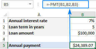
Tip. To calculate the total amount paid for the loan, multiply the returned PMT value by the number of periods (nper value). In our case, we'd use this equation: 24,389.07*5 and find that the total amount equals $121,945.35.
How to use PMT function in Excel - formula examples
Below you will find a few more examples of an Excel PMT formula that show how to calculate different periodic payments for a car loan, home loan, mortgage loan, and the like.
Full form of PMT function in Excel
For the most part, you can omit the last two arguments in your PMT formulas (like we did in the above examples) because their default values cover the most typical uses cases:
- Fv omitted - implies zero balance after the last payment.
- Type omitted - payments are due at the end of each period.
If your loan conditions are different from the defaults, then use the full form of PMT formula.
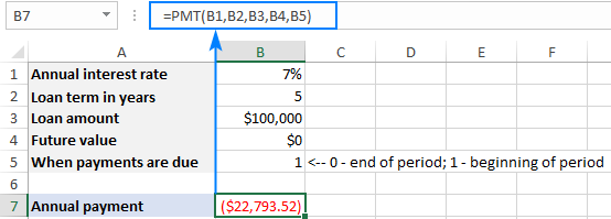
As an example, let's calculate the amount of annual payments based on these input cells:
- B1 - annual interest rate
- B2 - loan term (in years)
- B3 - loan amount
- B4 - future value (balance after the last payment)
- B5 - annuity type:
- 0 (regular annuity) - payments are made at the end of each year.
- 1 (annuity due) - payments are made at the beginning of the period, e.g. rent or lease payments.
Supply these references to your Excel PMT formula:
=PMT(B1, B2, B3, B4, B5)
And you will have this result:
Calculate weekly, monthly, quarterly and semi-annual payments
Depending on the payment frequency, you need to use the following calculations for rate and nper arguments:
- For rate, divide the annual interest rate by the number of payments per year (which is deemed to be equal to the number of compounding periods).
- For nper, multiply the number of years by the number of payments per year.
The below table provides the details:
| Payment Frequency | Rate | Nper |
| Weekly | annual interest rate / 52 | years * 52 |
| Monthly | annual interest rate / 12 | years * 12 |
| Quarterly | annual interest rate / 4 | years * 4 |
| Semi-annual | annual interest rate / 2 | years * 2 |
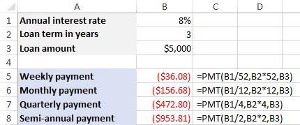
For instance, to find the amount of a periodic payment on a $5,000 loan with an 8% annual interest rate and a duration of 3 years, use one of the below formulas.
Weekly payment:
=PMT(8%/52, 3*52, 5000)
Monthly payment:
=PMT(8%/12, 3*12, 5000)
Quarterly payment:
=PMT(8%/4, 3*4, 5000)
Semi-annual payment:
=PMT(8%/2, 3*2, 5000)
In all cases, the balance after the last payment is assumed to be $0, and the payments are due at the end of each period.
The screenshot below shows the results of these formulas:
How to make a PMT calculator in Excel
Before you go ahead and borrow money, it stands to reason to compare different loan conditions to find out the options that suit you most. For this, let's create our own Excel loan payment calculator.
- To begin with, enter the loan amount, interest rate and loan term in separate cells (B3, B4, B5, respectively).
- To be able to choose different periods and specify when the payments are due, create drop-down lists with the following predefined options (B6 and B7):

- Set up the lookup tables for Periods (E2:F6) and Payments are Due (E8:F9) like show in the screenshot below. It is important that text labels in the lookup tables exactly match the items of the corresponding drop-down list.
In the cells next to the drop-down lists, enter the following IFERROR VLOOKUP formulas that will pull the number from the lookup table corresponding to the item selected in the drop-down list.Formula for Periods (C6):
=IFERROR(VLOOKUP(B6, E2:F6, 2, 0), "")Formula for Payments are Due (C7):
=IFERROR(VLOOKUP(B7, E8:F9, 2, 0), "")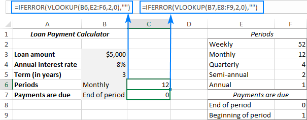
- Write a PMT formula to calculate the periodic payment based on your cells. In our case, the formula goes as follows:
=IFERROR(-PMT(B4/C6, B5*C6, B3, 0, C7), "")Please notice the following things:
- The fv argument (0) is hardcoded in the formula because we always want zero balance after the last payment. In case you wish to allow your users to enter any future value, allocate a separate input cell for the fv argument.
- The PMT function is preceded with the minus sign to display the result as a positive number.
- The PMT function is wrapped into IFERROR to hide errors when some input values are not defined.
The above formula goes in B9. And in the neighboring cell (A9) we display a label corresponding to the selected period (B6). For this, simply concatenate the value in B6 and the desired text:
=B6&" Payment"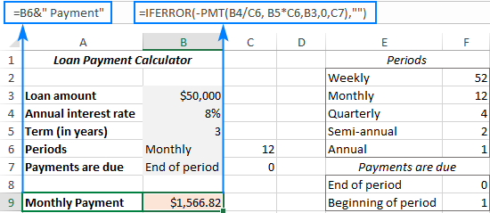
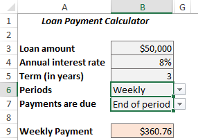
- Finally, you can hide the lookup tables from view, add a few finishing formatting touches, and your Excel PMT calculator is good to go:
Excel PMT function not working
If your Excel PMT formula is not working or produces wrong results, it's likely to be because of the following reasons:
- A #NUM! error may occur if either the rate argument is a negative number or nper is equal to 0.
- A #VALUE! error occurs if one or more arguments are text values.
- If the result of a PMT formula is much higher or lower than expected, make sure you are consistent with the units supplied for the rate and nper arguments, meaning you have correctly converted the annual interest rate to the period's rate and the number of years to weeks, months, or quarters as shown in this example.
That's how you calculate PMT function in Excel. To have a closer look at the formulas discussed in this tutorial you are welcome to download our sample workbook below. I thank you for reading and hope to see you on our blog next week!
Practice workbook for download
PMT formula in Excel - examples(.xlsx file)
 by
by
24 comments
Great tool and great help. I highly appreciate your explanation method. I want to make a request to you.
Now adays many people invest in mutual funds via ‘Step Up SIP’ method. In this method, monthly investment amount increases every year by a certain percentage or by certain amount, as decided by the investor. There is no direct function in excel for step up SIP calculation. Pl make excel sheet / formula to calculate followings, in case of Step Up SIP investment along with lump sum investment.
FV, PV, Rate, Nper, PMT ect.
Thanks and regards,
SK Sharma
Great tool and great help. I highly appreciate your explanation method. I want to make one request to you.
Now a days many people invest in mutual fund via 'Step Up SIP' method. In this method, monthly investment amount increases every year by a certain percentage or certain amount as decided by the investor. There is no function in excel to calculate 'step Up SIP'. Pl. make excel sheets which may calculate followings in case of investment via 'step up SIP' method and an initial lump sum amount.
FV, PV, Rate, Nper, PMT ect.
Thank and regard.
SK Sharma
Use the PMT function in Excel to compute the monthly payment on a car each month if you borrowed $7700 at an annual interest rate of 4.73% over 4 years, where the interest is compounded monthly.
Really Appreciated, Very Useful and direct to the point
Thank you Very much for the support
Can you please help me to get the monthly payment?
Lease
Price of Car $25,000
Residual Value $15,000
Interest Rate(per Year) 7.0%
Terms of Loan (years) 3
Monthly Payment ????
Hi, Good day,
May I know is it ok to apply Nper with decimal positions? for example: 8/3
Sample Case:
Loan Term: 8 Months,
the first 2 Term: Quarterly Basis
the remaining 2 Term is Monthly Basis
Quarterly Payment: 1,944.13 =PMT(8%/12*3, 8/3, -5,000)
Monthly Payment: 643.81 =PMT(8%/12, 2, -1,274.86)
(1274.86 = 5,000 - the Principal of the first 2 terms)
Thank you,
For example, if you borrow $100,000 for 5 years with an annual interest rate of 7%, the following formula will calculate the annual payment:
=PMT(7%, 5, 100000)
($24,389.07) <-- THIS IS THE ANSWER I GET IN EXCEL
To find the monthly payment for the same loan, use this formula:
=PMT(7%/12, 5*12, 100000)
($1,980.12) <-- THIS IS THE ANSWER I GET IN EXCEL
THESE DO NOT CHECK OUT!
Divide 24,389.07 by 12 = $2,032.42 <-- Does NOT equal the monthly.
Multiply 1,980.12 by 12 = $23,761.44 <-- Does NOT equal the annual.
SOMETHING IS WRONG! Can you please clarify? Thank you.
Hello! This function calculates an annuity payment, where you pay a fixed amount of money for a loan on a regular basis. These amounts cannot and should not be equal! When you repay the loan in installments, you pay less, because the remaining balance of the loan decreases with each payment, and interest depends on it.
Mike,
The discrepancy is due to compounding. With the annual payment scenario of your first example, you're incurring an entire year's worth of interest before making that first of five annual payments. After you make that first annual payment, a portion is applied to the principal and a portion is assigned to interest. Thereafter, your principal is reduced by the amount of the first payment applied to the principal. During the second year of the loan, the remaining principal amount is subjected to an entire year's worth (7% in your example) of interest. Then you make the second annual payment and the process repeats.
The in the monthly payment scenario, the same process plays out, but it is more rapid because you're paying on a monthly basis. That means that every month you make a payment, a portion goes to principal and a portion goes to interest. For the second month, your remaining loan balance is reduced by the amount of the monthly payment you just made that went to principal. There's the source of the difference. With the monthly payment plan, you're chipping away at the principal (the remaining loan balance) every single month. The result is that every month the remaining loan balance is lower and only subjected to interest expense for one month. Then you make the second monthly payment and lower your principal (remaining loan balance) yet again. Now the interest rate is applied to a lower loan balance, because you just made your second monthly payment and reduced your loan balance.
To summarize, with monthly payments, you're reducing your loan balance more rapidly because part of your monthly payment goes toward reducing the loan balance. That leaves a lower balance that interest is charged against. When you're making annual payments, the loan balance sit for an entire year before it gets reduced by your annual payment. Sitting there for an entire year means your interest expense are building up and more of your annual payment will go toward interest expense.
Making 5 annual payments of $24,389.07 means you'll pay a total of $121,945.35 to repay your 7%, $100,000 loan over five years.
Making 5 * 12 = 60 monthly payments of $1,980.12 means you'll pay a total of $118,807.19 to repay that same 7%, %100,000 loan over sixty months.
This is why some financial advisors advise clients to repay their home mortgages with 26 biweekly payments, instead of 12 monthly payments. By accelerating the payment schedule, even with the same overall payment amount, more of your money is going towards paying down the principal and less is going towards interest expenses. Hope this helps! Best wishes.
How do i separate the interest and amortisation numbers?
If I want the loan to be repaid in less than a year; and the frequency of payment is weekly, then what are the changes required to the formula?
Well, I'd like to know the maths behind the formula. Because I can use the formula and I can accept it's correct but if we put the formula to one side and I suppose I have a $12,000 loan to be repaid monthly over a 2 year period and the interest rate is 12% APR then without using the PMT formula how do I arrive at your answer? What the mathematical model behind the formula. I just can't make any sense of it. The way I reasoned it was:
The person will pay 1% interest a month and will pay the interest plus $500 repayment of the capital. So at the end of the first month the person pays back $500 + $120 (interest) or $620 in all. There is now $11,500 left to be repaid and we process this calculation again but in the end the two figures don't agree. I accept I've got the wrong model in my head but then I can't work out how the model is working and why it's accurate - if you see what I mean? Never mind too much, I just got to use the formula and never mind the maths so much :).
How do you make use of PMT where the first loan repayment is for a different period to the other repayments. This often happens with consumer loans to allow a repayment program that matches the borrowers income stream
How to calculate a monthly rate of PMT?
It is so good greatful knowledge i like it very much
Good in-depth explanation of such complex formula. I have now got a complete grip on the same. Thanks for sharing the knowledge and keep up the good work.
Does anyone know how to calculate an amount per period over a period of 3 months using a formula on excel?
for this PMT, if I use manual count. I can't get the same amount like the PMT amount shown. How?
PMT IN ECXEL FULL FORM
Hi, just to check something come out from my mind. My question is about letter of credit. What if the banker interest rate is totally diff in each of every month what do I work out from PMT formula.
Then we also need to get back whatever is gain.
Thank you
Does anyone know how to calculate an auto lease in access using a pmt formula?
ms excel 7.0 version formula lab a to z exprience in hindi
Hi Karna,
The full form of PMT is described in this tutorial. The full forms of the other two functions can be found here:
Full form of PPMT formula
Full form of IPMT formula
Kindly let us know full form of PMT, PPMT, IPMT.
Please,
Thanks.