The tutorial shows three different ways to hide rows in your worksheets. It also explains how to show hidden rows in Excel and how to copy only visible rows.
If you want to prevent users from wandering into parts of a worksheet you don't want them to see, then hide such rows from their view. This technique is often used to conceal sensitive data or formulas, but you may also wish to hide unused or unimportant areas to keep your users focused on relevant information.
On the other hand, when updating your own sheets or exploring inherited workbooks, you would certainly want to unhide all rows and columns to view all data and understand the dependencies. This article will teach you both options.
How to hide rows in Excel
As is the case with nearly all common tasks in Excel, there is more than one way to hide rows: by using the ribbon button, right-click menu, and keyboard shortcut.
Anyway, you begin with selecting the rows you'd like to hide:
- To select one row, click on its heading.
- To select multiple contiguous rows, drag across the row headings using the mouse. Or select the first row and hold down the Shift key while selecting the last row.
- To select non-contiguous rows, click the heading of the first row and hold down the Ctrl key while clicking the headings of other rows that you want to select.
With the rows selected, proceed with one of the following options.
Hide rows using the ribbon
If you enjoy working with the ribbon, you can hide rows in this way:
- Go to the Home tab > Cells group, and click the Format button.
- Under Visibility, point to Hide & Unhide, and then select Hide Rows.
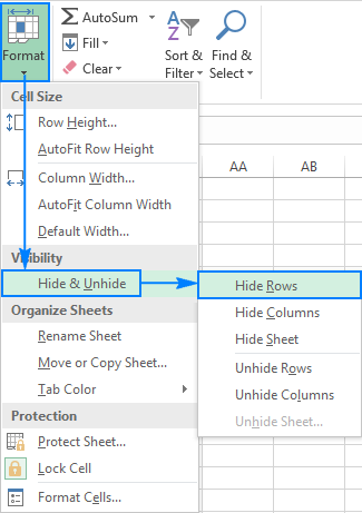
Alternatively, you can click Home tab >Format > Row Height… and type 0 in the Row Height box.
Either way, the selected rows will be hidden from view straight away.
Hide rows using the right-click menu
In case you don't want to bother remembering the location of the Hide command on the ribbon, you can access it from the context menu: right click the selected rows, and then click Hide.
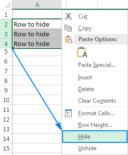
Excel shortcut to hide row
If you'd rather not take your hands off the keyboard, you can quickly hide the selected row(s) by pressing this shortcut: Ctrl + 9
How to unhide rows in Excel
As with hiding rows, Microsoft Excel provides a few different ways to unhide them. Which one to use is a matter of your personal preference. What makes the difference is the area you select to instruct Excel to unhide all hidden rows, only specific rows, or the first row in a sheet.
Unhide rows by using the ribbon
On the Home tab, in the Cells group, click the Format button, point to Hide & Unhide under Visibility, and then click Unhide Rows.
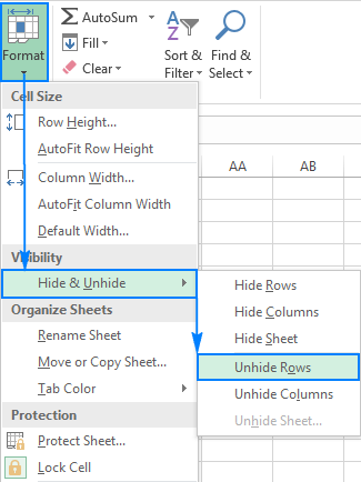
Unhide rows using the context menu
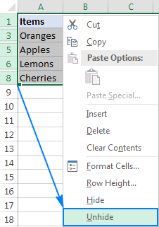
You select a group of rows including the row above and below the row(s) you want to unhide, right-click the selection, and choose Unhide in the pop-up menu. This method works beautifully for unhiding a single hidden row as well as multiple rows.
For example, to show all hidden rows between rows 1 and 8, select this group of rows like shown in the screenshot below, right-click, and click Unhide:
Unhide rows with a keyboard shortcut
Here is the Excel Unhide Rows shortcut: Ctrl + Shift + 9
Pressing this key combination (3 keys simultaneously) displays any hidden rows that intersect the selection.
Show hidden rows by double-clicking
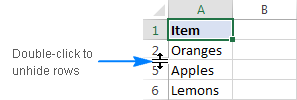
In many situations, the fastest way to unhide rows in Excel is to double click them. The beauty of this method is that you don't need to select anything. Simply hover your mouse over the hidden row headings, and when the mouse pointer turns into a split two-headed arrow, double click. That's it!
How to unhide all rows in Excel
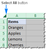
In order to unhide all rows on a sheet, you need to select all rows. For this, you can either:
- Click the Select All button (a little triangle at the upper left corner of a sheet, in the intersection of the row and column headings):
- Press the Select All shortcut: Ctrl + A
Please note that in Microsoft Excel, this shortcut behaves differently in different situations. If the cursor is in an empty cell, the whole worksheet is selected. But if the cursor is in one of contiguous cells with data, only that group of cells is selected; to select all cells, press Ctrl+A one more time.
Once the entire sheet is selected, you can unhide all rows by doing one of the following:
- Press Ctrl + Shift + 9 (the fastest way).
- Select Unhide from the right-click menu (the easiest way that does not require remembering anything).
- On the Home tab, click Format > Unhide Rows (the traditional way).
How to unhide all cells in Excel
To unhide all rows and columns, select the whole sheet as explained above, and then press Ctrl + Shift + 9 to show hidden rows and Ctrl + Shift + 0 to show hidden columns.
How to unhide specific rows in Excel
Depending on which rows you want to unhide, select them as described below, and then apply one of the unhide options discussed above.
- To show one or several adjacent rows, select the row above and below the row(s) that you want to unhide.
- To unhide multiple non-adjacent rows, select all the rows between the first and last visible rows in the group.
For example, to unhide rows 3, 7, and 9, you select rows 2 - 10, and then use the ribbon, context menu or keyboard shortcut to unhide them.
How to unhide top rows in Excel
Hiding the first row in Excel is easy, you treat it just like any other row on a sheet. But when one or more top rows are hidden, how do you make them visible again, given that there is nothing above to select?
The clue is to select cell A1. For this, just type A1 in the Name Box, and press Enter.
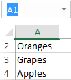
Alternatively, go to the Home tab > Editing group, click Find & Select, and then click Go To… . The Go To dialog window pops up, you type A1 in the Reference box, and click OK.
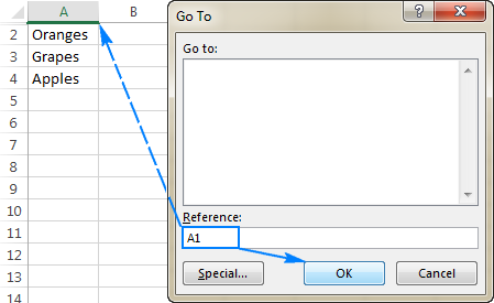
With cell A1 selected, you can unhide the first hidden row in the usual way, by clicking Format > Unhide Rows on the ribbon, or choosing Unhide from the context menu, or pressing the unhide rows shortcut Ctrl + Shift + 9
Aside from this common approach, there is one more (and faster!) way to unhide first row in Excel. Simply hover over the hidden row heading, and when the mouse pointer turns into a split two-headed arrow, double click:

Tips and tricks for hiding and unhiding rows in Excel
As you have just seen, hiding and showing rows in Excel is quick and straightforward. In some situations, however, even a simple task can become a challenge. Below you will find easy solutions to a few tricky problems.
How to hide rows containing blank cells
To hide rows that contain any blank cells, proceed with these steps:
- Select the range that contains empty cells you want to hide.
- On the Home tab, in the Editing group, click Find & Select > Go To Special.
- In the Go To Special dialog box, select the Blanks radio button, and click OK. This will select all empty cells in the range.
- Press Ctrl + 9 to hide the corresponding rows.
This method works well when you want to hide all rows that contain at least one blank cell, as shown in the screenshot below:

If you want to hide blank rows in Excel, i.e. the rows where all cells are blank, then use the COUNTBLANK formula explained in How to remove blank rows to identify such rows.
How to hide rows based on cell value
To hide and show rows based on a cell value in one or more columns, use the capabilities of Excel Filter. It provides a handful of predefined filters for text, numbers and dates as well as an ability to configure a custom filter with your own criteria (please follow the above link for full details).
To unhide filtered rows, you remove filter from a specific column or clear all filters in a sheet, as explained here.
Hide unused rows so that only working area is visible
In situations when you have a small working area on the sheet and a whole lot of unnecessary blank rows and columns, you can hide unused rows in this way:
- Select the row beneath the last row with data (to select the entire row, click on the row header).
- Press Ctrl + Shift + Down arrow to extend the selection to the bottom of the sheet.
- Press Ctrl + 9 to hide the selected rows.
In a similar fashion, you hide unused columns:
- Select an empty column that comes after the last column of data.
- Press Ctrl + Shift + Right arrow to select all other unused columns to the end of the sheet.
- Press Ctrl + 0 to hide the selected columns. Done!
If you decide to unhide all cells later, select the entire sheet, then press Ctrl + Shift + 9 to unhide all rows and Ctrl + Shift + 0 to unhide all columns.
How to locate all hidden rows on a sheet
If your worksheet contains hundreds or thousands of rows, it can be hard to detect hidden ones. The following trick makes the job easy.
- On the Home tab, in the Editing group, click Find & Select > Go To Special. Or press Ctrl+G to open the Go To dialog box, and then click Special.
- In the Go To Special window, select Visible cells only and click OK.
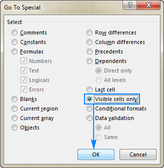
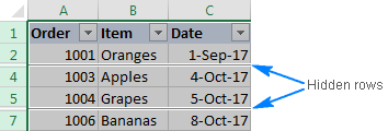
This will select all visible cells and mark the rows adjacent to hidden rows with a white border:
How to copy visible rows in Excel
Supposing you have hidden a few irrelevant rows, and now you want to copy the relevant data to another sheet or workbook. How would you go about it? Select the visible rows with the mouse and press Ctrl + C to copy them? But that would also copy the hidden rows!
To copy only visible rows in Excel, you'll have to go about it differently:
- Select visible rows using the mouse.
- Go to the Home tab > Editing group, and click Find & Select > Go To Special.
- In the Go To Special window, select Visible cells only and click OK. That will really select only visible rows like shown in the previous tip.
- Press Ctrl + C to copy the selected rows.
- Press Ctrl + V to paste the visible rows.
Cannot unhide rows in Excel
If you have troubles unhiding rows in your worksheets, it's most likely because of one of the following reasons.
1. The worksheet is protected
Whenever the Hide and Unhide features are disabled (greyed out) in your Excel, the first thing to check is worksheet protection.
For this, go to the Review tab > Changes group, and see if the Unprotect Sheet button is there (this button appears only in protected worksheets; in an unprotected worksheet, there will be the Protect Sheet button instead). So, if you see the Unprotect Sheet button, click on it.
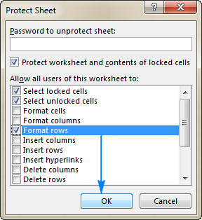
If you want to keep the worksheet protection but allow hiding and unhiding rows, click the Protect Sheet button on the Review tab, select the Format rows box, and click OK.
Tip. If the sheet is password-protected, but you cannot remember the password, follow these guidelines to unprotect worksheet without password.
2. Row height is small, but not zero
In case the worksheet is not protected but specific rows still cannot be unhidden, check the height of those rows. The point is that if a row height is set to some small value, between 0.08 and 1, the row seems to be hidden but actually it is not. Such rows cannot be unhidden in the usual way. You have to change the row height to bring them back.
To have it done, perform these steps:
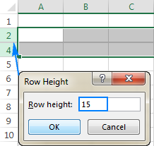
- Select a group of rows, including a row above and a row below the problematic row(s).
- Right click the selection and choose Row Height… from the context menu.
- Type the desired number of the Row Height box (for example the default 15 points) and click OK.
This will make all hidden rows visible again.
If the row height is set to 0.07 or less, such rows can be unhidden normally, without the above manipulations.
3. Trouble unhiding the first row in Excel
If someone has hidden the first row in a sheet, you may have problems getting it back because you cannot select the row before it. In this case, select cell A1 as explained in How to unhide top rows in Excel and then unhide the row as usual, for example by pressing Ctrl + Shift + 9.
4. Some rows are filtered out
When the row numbers in your worksheet turn blue, this indicates that some rows are filtered out. To unhide such rows, simply remove all filters on a sheet.
This is how you hide and undie rows in Excel. I thank you for reading and hope to see you on our blog next week!
 by
by
39 comments
In my Excel sheet, I have unhidden the hidden rows from 1 to 346 but I have observed that after unhiding rows still when I right-click the unhide option is not greyed out and appears. I have tried multiple times but it appears the same even though there are now rows hidden. Please let me know if there is any solution for this
Hi! I really have no idea what your problem is. If you use the Unhide option for the rows that are not hidden, nothing will be changed in your worksheet.
Agree! But my question is, why is the 'Unhide' option not greyed out when there are no rows hidden
That's a question that should be asked of Microsoft.
For some reason, not a single one of those solutions had any effect, except for me individually double-clicking each hidden row, but this runs the risk that I might miss one because there are hundreds of hidden rows in my messed-up file.
Excel = cancer for having this broken anti-feature.
Nothing worked. On a lark, I decided to unfreeze panes and the rows popped into view!.
Thank you, this is exactly what i was looking for!!
Best cheatsheat/tutorial in my opinion out there in the vast expanse today. Thanks!
Just wanted to say thank you very much. Your help is highly appreciated.
I couldn't get many of the things working (and I've gone through quite a sites through), but double-clicking worked... thanks!
Unfortunately, none of it worked for me; Unable to unhide initial rows :-(
Be sure to turn off any filters!
Molly you need to group the columns or rows.
Go to Data tab, at far right you will see Group, Ungroup icons.
First click on the columns or row headings, then click on Group or ungroup if you want to amend the areas to hide.
I have a worksheet where colA is hidden and rows 1-3 are hidden. I don't know how it happened. I have tried all the above and nothing works. Can anyone help.
How do you hide rows but display the "+" so they can be un-hidden/re-hidden just by clicking on the + or - ???
...that's for Pivot tables
...no it's not.
I believe this is the way:
- Select the columns or rows you are interested in hiding -> Go to Data tab -> Go to Outline -> Click on Gorup
Thank you Zuzana! You had the solution I was looking for :D
How to hide row or column with condition
I am an AbleBits very satisfied customer but none of the tips on how to unhide rows at the top of my worksheet have worked.
Hi Gail,
Try selecting the entire sheet (Ctrl+A), right-click any row and select "Unhide". If this does not work, then most likely the rows are filtered out. In this case, simply clear all the filters (Home tab > Editing group > Sort & Filter > Clear).
Hi Svetlana ; 'Filters cleared and problem solved' - thanks
Great... Thank you so much...it works
Thank you very much. U have helped a lot...Best solution ever...
I've managed to hide rows but once I pressed save I can't unhide them. Am I missing something?
I'm glad I read to the end!
I had most of my sheet hidden and none of the above mentioned worked until I selected the entire sheet and cleared the filters. Thank you for the article.
I found it is easy to accidentally hide all rows and columns if I click the right corner arrow and highlight the entire worksheet and hit hide. I know this is not correct, but it can happen. I could not find any advice on how to fix the problem so I worked it out for myself. If I had the curse on the row column, I just hovered the cursor to the left of the corner arrow until the two lines appeared, and right clicked and selected "Unhide". If I hide the cursor on the columns row when I hid the entire sheet, I hovered the cursor between the corner arrow and the column row to get the dual lines and right clicked and selected "Unhide". If there are any other Excel users who have had this problem, they may appreciate this little bit of information.
Thank you very much. very helpful :)
Is it possible to automatically hide using a formula, for example
Opening balance:
Account balance:
Total :
If no opening balance exists then is it possible to automatically hide this cell so it will now say
Account balance:
Total:
I am trying to automate a spreadsheet so that on the "workbook" someone only needs to input the figures but on the "notice" it will auto format to show just the relevant information.
Thank you
see above:
How to hide rows based on cell value
To hide and show rows based on a cell value in one or more columns, use the capabilities of Excel Filter. It provides a handful of predefined filters for text, numbers and dates as well as an ability to configure a custom filter with your own criteria (please follow the above link for full details).
To unhide filtered rows, you remove filter from a specific column or clear all filters in a sheet, as explained here
how to count total number of sheets in a excel workbook
how to delete blank rows in my excel data except rows that aren't completely blank
Amazing, the most comprenhensive information I have found, one of the tips solved my problem. Thanks a lot!
Thank you very much for this information. Always appreciate those who extend the effort to those who wish to learn.
Roy
I have 530 rows hidden and I don't want to sit and double click 530 times to unhide ALL of them. Is there not a way to unhide a rediculous number of hidden rows all at once?
I have same problem. I still cannot unhide Rows even I have done every steps in this suggestion.
Use CTRl+Home on your keyboard. Then left-click the gray box that has the bottom right-corner arrow in it (found directly under the A1 cell name box). This will select the entire worksheet. Move cursor over any Row Number and right-click, then select Unhide. You can do the same to Unhide all columns - just move cursor over a column letter and right-click.
Thanks a lot it works. I have tried.
No???