Today we'll take a close look at the syntax and typical uses of the new dynamic array SORTBY function. You will learn how to custom sort in Excel with a formula, randomly sort a list, arrange cells by text length, and more.
Microsoft Excel provides a number of ways to arrange text data alphabetically, dates chronologically, and numbers from smallest to largest or from highest to lowest. There is also a way to sort by your own custom lists. In addition to the conventional Sort functionality, Excel 365 introduces a brand-new way to sort data with formulas - very convenient and incredibly simple to use!
Excel SORTBY function
The SORTBY function in Excel is designed to sort one range or array based on the values in another range or array. Sorting can be done by one or multiple columns.
SORTBY is one of six new dynamic array functions available in Excel for Microsoft 365 and Excel 2021. Its result is a dynamic array that spills to neighboring cells and updates automatically when the source data changes.
The SORTBY function has a variable number of arguments - the first two are required and the other are optional:
Array (required) - the range of cells or array of values to be sorted.
By_array1 (required) - the range or array to sort by.
Sort_order1 (optional) - the sorting order:
- 1 or omitted (default) - ascending
- -1 - descending
By_array2 / Sort_order2, … (optional) - additional array / order pairs to use for sorting.
Important note! Currently the SORTBY function is only available with Microsoft 365 subscriptions and Excel 2021. In Excel 2019, Excel 2016 and earlier versions the SORTBY function is not available.
SORTBY function - 4 things to remember
For an Excel SORTBY formula to work correctly, there are a few important points to take notice of:
- By_array arguments should be either one row high or one column wide.
- The array and all by_array arguments must have compatible dimensions. For example, when sorting by two columns, array, by_array1 and by_array2 should have the same number of rows; otherwise a #VALUE error will occur.
- If the array returned by SORTBY is the final result (output in a cell and not passed to another function), Excel creates a dynamic spill range and populates it with the results. So, be sure you have enough empty cells down and/or to the right of the cell where you enter the formula, otherwise you'll get a #SPILL error.
- The results of SORTBY formulas update automatically whenever the source data changes. However, new entries that are added outside of the array referenced in the formula are not included in the results unless you update the array reference. For the referenced array to expand automatically, convert the source range to an Excel table or create a dynamic named range.
Basic SORTBY formula in Excel
Here's a typical scenario of using a SORTBY formula in Excel:
Supposing, you have a list of projects with the Value field. You want to sort the projects by their value on a separate sheet. As other users do not need to see the numbers, you'd rather not include the Value column in the results.
The task can be easily accomplished with the SORTBY function, for which you supply the following arguments:
- Array is A2:A10 - since you do not wish the Value column to be displayed in the results, you leave it out of the array.
- By_array1 is B2:B10 - sort by Value.
- Sort_order1 is -1 - descending, i.e. from highest to lowest.
Putting the arguments together, we get this formula:
=SORTBY(A2:B10, B2:B10, -1)
For simplicity, we use the formula on the same sheet - enter it in D2 and press the Enter key. The results "spill" automatically to as many cells as needed (D2:D10 in our case). But technically, the formula is only in the first cell, and deleting it from D2 will delete all the results.
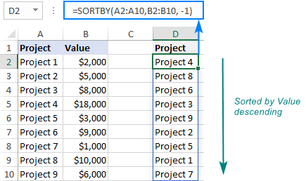
When used on another sheet, the formula takes the following shape:
=SORTBY(Sheet1!A2:A10, Sheet1!B2:B10, -1)
Where Sheet1 is the worksheet containing the original data.
Using SORTBY function in Excel - formula examples
Below you will find a few more examples of using SORTBY, which will hopefully prove useful and insightful.
Sort by multiple columns
The basic formula discussed above sorts data by one column. But what if you need to add one more level of sorting?
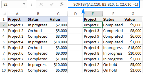
Assuming our sample table has two fields, Status (column B) and Value (column C), we wish to sort first by Status alphabetically, and then by Value descending.
To sort by two columns, we just add one more pair of the by_array / sort_order arguments:
- Array is A2:C10 - this time, we want to include all three columns in the results.
- By_array1 is B2:B10 - first, sort by Status.
- Sort_order1 is 1 - sort alphabetically from A to Z.
- By_array2 is C2:C10 - then, sort by Value.
- Sort_order2 is -1 - sort from largest to smallest.
As the result, we get the following formula:
=SORTBY(A2:B10, B2:B10, 1, C2:C10, -1)
Which rearranges our data exactly as we instructed it:
Custom sort in Excel with a formula
To sort data in a custom order, you can either use Excel's Custom Sort feature or build a SORTBY MATCH formula in this way:
Taking a closer look at our data set, you will probably find it more convenient to sort the projects by their status "logically", e.g. by importance, rather than alphabetically.
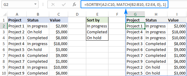
To have it done, we first create a custom list in the desired sort order (In progress, Completed, On hold) typing each value in a separate cell in the range E2:E4.
And then, using the generic formula above, we supply the source range for array (A2:C10), the Status column for range_to_sort (B2:B10), and the custom list that we created for custom_list (E2:E4).
=SORTBY(A2:C10, MATCH(B2:B10, E2:E4, 0))
As the result, we've got the projects sorted by their status exactly as needed:
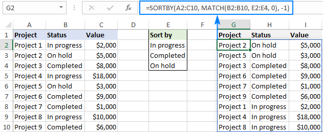
To sort by custom list in the reverse order, put -1 for the sort_order1 argument:
=SORTBY(A2:C10, MATCH(B2:B10, E2:E4, 0), -1)
And you'll have the projects sorted in the opposite direction:
Want to additionally sort records within each status? No problem. Simply, add one more sort level to the formula, say by Value (C2:C10), and define the desired order of sorting, ascending in our case:
=SORTBY(A2:C10, MATCH(B2:B10, E2:E5, 0), 1, C2:C10, 1)
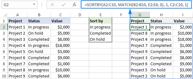
A big advantage of the SORTBY formula over Excel's Custom Sort feature is that the formula updates automatically whenever the original data changes, while the feature requires cleaning up and re-sorting with each change.
How this formula works:
As already mentioned, Excel's SORTBY function can only process "sort by" arrays whose dimensions are compatible with the source array. As our source array (C2:C10) contains 9 rows and the custom list (E2:E4) only 3 rows, we cannot supply it directly to the by_array argument. Instead, we use the MATCH function to create a 9-row array:
MATCH(B2:B10, E2:E5, 0)
Here, we use the Status column (B2:B10) as lookup values and our custom list (E2:E5) as lookup array. The last argument is set to 0 to look for exact matches. As the result, we get an array of 9 numbers, each representing the relative position of a given Status value in the custom list:
{1;3;2;1;3;2;2;1;2}
This array goes directly to the by_array argument of the SORTBY function and forces it to place the data in the order corresponding to the elements of the array, i.e. first entries represented by 1's, then entries represented by 2's, and so on.
Random sort in Excel with a formula
In earlier Excel versions, you can do a random sort with the RAND function as explained in this tutorial: How to randomly sort a list in Excel.
In new Excel, you can use a more powerful RANDARRAY function together with SORTBY:
Where array is the source data that you want to shuffle.
This generic formula works for a list consisting of a single column as well as for a multi-column range.
For example, to randomly sort a list in A2:A10, use this formula:
=SORTBY(A2:A10, RANDARRAY(ROWS(A2:A10)))
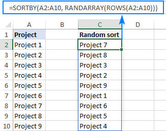
To shuffle data in A2:C10 keeping the rows together, use this one:
=SORTBY(A2:C10, RANDARRAY(ROWS(A2:C10)))
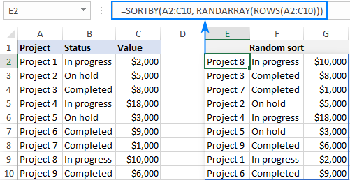
How this formula works:
The RANDARRAY function produces an array of random numbers to be used for sorting, and you pass it in the by_array argument of SORTBY. To specify how many random numbers to generate, you count the number of rows in the source range by using the ROWS function, and "feed" that number to the rows argument of RANDARRAY. That's it!
Note. Like its predecessor, RANDARRAY is a volatile function and it generates a new array of random numbers every time the worksheet is recalculated. As the result, your data will be resorted with each change on the sheet. To prevent auto resorting, you can use the Paste Special > Values feature to replace formulas with their values.
Sort cells by string length
To sort cells by the length of text strings they contain, use the LEN function to count the number of characters in each cell, and supply the calculated lengths to the by_array argument of SORTBY. The sort_order argument can be set to either 1 or -1, depending on the preferred order of sorting.
To sort by text string from smallest to largest:
To sort by text string from largest to smallest:
And here's a formula that demonstrates this approach on real data:
=SORTBY(A2:A7, LEN(A2:A7), 1)
Where A2:A7 are the original cells you'd like to sort by text length in ascending order:
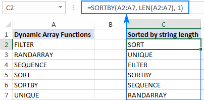
SORTBY vs. SORT
In the group of new Excel dynamic array functions, there are two designed for sorting. Below we list the most essential differences and similarities as well as when each is best to be used.
- Unlike the SORT function, SORTBY does not require the "sort by" array to be part of the source array, nor does it need to appear in results. So, when your task is to sort a range based on another independent array or a custom list, SORTBY is the right function to use. If you are looking to sort a range based on its own values, then SORT is more appropriate.
- Both functions support multiple levels of sorting and both can be chained together with other dynamic array and conventional functions.
- Both functions are only available to Excel 365 and Excel 2021 users.
Excel SORTBY function not working
In case your SORTBY formula returns an error, it's most likely because of one of the following reasons.
Invalid by_array arguments
The by_array argument must be a single row or a single column and compatible in size with the array argument. For example, if array has 10 rows, by_array should also include 10 rows. Otherwise a #VALUE! error occurs.
Invalid sort_order arguments
The sort_order arguments can only be 1 (ascending) or -1 (descending). If no value is set, SORTBY defaults to ascending order. If any other value is set, a #VALUE! error is returned. For more information, see When is #VALUE error raised in Excel?
There isn't enough space for results
Like any other dynamic array function, SORTBY spills the results into an automatically resizable and updatable range. If there are not enough empty cells to display all values, a #SPILL! error is thrown.
Source workbook is closed
If a SORTBY formula references another Excel file, both workbooks need to be open. If the source workbook is closed, a #REF! error occurs.
Your Excel version does not support dynamic arrays
When used in a pre-dynamic version of Excel, the SORT function returns a #NAME? error.
That's how to use the SORTBY function in Excel to do custom sort and other things. I thank you for reading and hope to see you on our blog next week!
Practice workbook for download
Excel SORTBY formulas (.xlsx file)
 by
by
5 comments
I want to use the Sort By function - i.e. Index and Match but i don't necessarily have a Custom Sort List. I just want to sort, say Stock scrips, with realized profit as value, in ascending order, dynamically. So i have NO custom list but your syntax looks like i have to mandatorily use a Custom list.. can i avoid it and just sort by Value?
Hi! You can sort values using Excel tools as described here: How to sort in Excel by row, column names and in custom order.
You can also use the SORT function. Look for the example formulas here: Excel SORT function - auto sort data using formula. I hope it’ll be helpful.
is there a way to sort by the url?
Example: I want to sort by URL abacustech.com
wrightn@ abacustech.com
Hi!
To sort email addresses by domain name, extract the domain name using the MID and SEARCH functions.
=SORTBY(A1:A4,MID(A1:A4,SEARCH("@",A1:A4)+1,20),1)
You can also find useful information in this article: Extract domain names from a URL list in Excel.
Hope this is what you need.
EXCELent!
Thank you for sharing.
And another usage of SORTBY function is:
Reverse an array:
=SORTBY(array, ROW(array),-1)