This tutorial will teach you a few quick and easy ways to put Excel in alphabetical order. It also provides solutions for non-trivial tasks, for example how to alphabetize by last name when the entries start with the first name.
Alphabetizing in Excel is as easy as ABC. Whether you are sorting an entire worksheet or selected range, vertically (a column) or horizontally (a row), ascending (A to Z) or descending (Z to A), in most cases the task can be accomplished with a button click. In some situations, however, the built-in features may stumble, but you can still figure out a way to sort by alphabetical order with formulas.
This tutorial will show you a few quick ways to alphabetize in Excel and teach how to foresee and prevent sorting problems.
How to alphabetize in Excel
Overall, there are 3 main ways to sort alphabetically in Excel: A-Z or Z-A button, the Sort feature, and filter. Below you will find the detailed guidance on each method.
How to sort a column alphabetically
The fastest way to sort alphabetically in Excel is this:
- Select any cell in the column you want to sort.
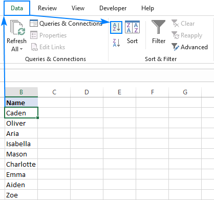
- On the Data tab, in the Sort and Filter group, click either A-Z to sort ascending or Z-A to sort descending. Done!
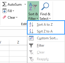
The same buttons can also be accessed from Home tab > Editing group > Sort and Filter:
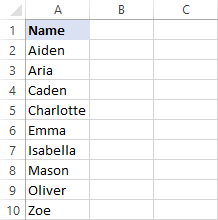
Either way, Excel will alphabetize your list instantaneously:
Tip. After you've done sorting and before you do anything else, take a close look at the results. If something looks wrong, click the Undo button to restore the original order.
Alphabetize and keep rows together
If your data set contains two or more columns, you can use the A-Z or Z-A button to put one of the columns in alphabetical order and Excel will automatically move the data in other columns, keeping the rows intact.
As you can see in the sorted table on the right, the related information in each row is kept together:
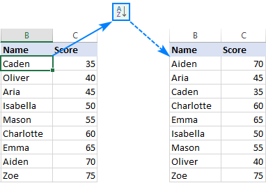
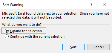
In some situations, mostly when just one or a few cells in the middle of your data set are selected, Excel is unsure which part of the data to sort and asks for your instructions. If you'd like to sort the entire dataset, leave the default Expand the selection option checked, and click Sort:
Note. In this tutorial, a "table" is just any data set. Technically, all our examples are for ranges. Excel table has inbuilt sorting and filtering options.
Filter and alphabetize in Excel
Another quick way to sort alphabetically in Excel is to add a filter. The beauty of this method is that it's one-time setup - once the auto filter is applied, the sort options for all columns are only a mouse click away.
Adding a filter to your table is easy:
- Select one or several column headers.
- On the Home tab, in the Editing group, click Sort and Filter > Filter.
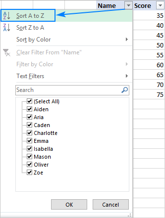
- Small drop-down arrows will appear in each of the column headers. Click the drop-down arrow for the column you want to put in alphabetical order, and select Sort A to Z:
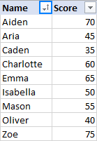
The column is alphabetized straight away, and a small upward arrow on the filter button indicates the sorting order (ascending):
To reverse the order, select Sort Z to A from the filter drop-down menu.
To remove the filter, simply click the Filter button again.
How to put multiple columns in alphabetical order
In case you want to alphabetize data in several columns, use the Excel Sort command, which gives more control over how your data is sorted.
As an example, let's add one more column to our dataset, and then arrange the entries alphabetically first by Region, and then by Name:
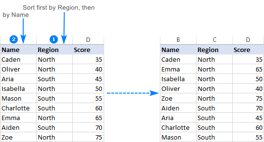
To have it done, please perform the following steps:
- Select the entire table you want to sort.
In most cases, you can select just one cell and Excel will pick the rest of your data automatically, but this is an error-prone approach, especially when there are some gaps (blank cells) within your data.
- On the Data tab, in the Sort & Filter group, click the Sort button.

- The Sort dialog box will show up with the first sorting level created for you automatically as Excel sees fit.
In the Sort by dropdown box, select the column you want to alphabetize first, Region in our case. In the other two boxes, leave the default settings: Sort On - Cell values and Order - A to Z:
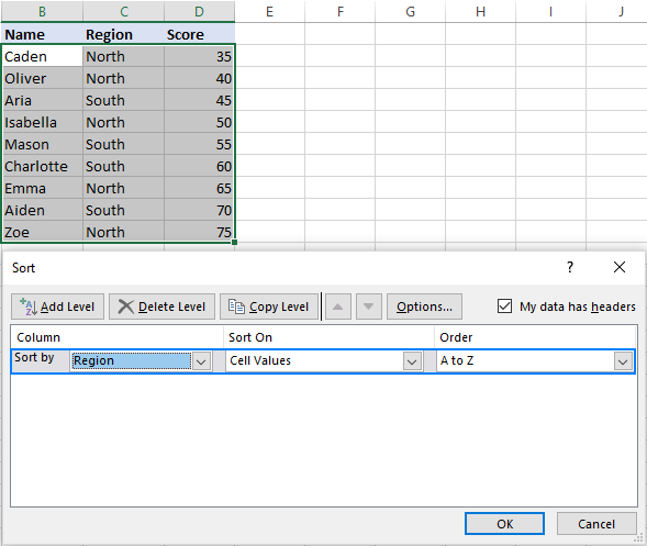
Tip. If the first dropdown is showing column letters instead of headings, tick off the My data has headers box.
- Click the Add Level button to add the next level and select the options for another column.
In this example, the second level sorts the values in the Name column alphabetically from A to Z:
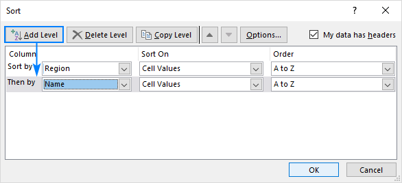
Tip. If you are sorting by multiple columns with the same criteria, click Copy Level instead of Add Level. In this case, you will only have to choose a different column in the first box.
- Add more sort levels if needed, and click OK.
Excel will sort your data in the specified order. As shown in the screenshot below, our table is arranged alphabetically exactly as it should: first by Region, and then by Name:
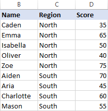
Tip. If the items you want to sort contain both text and numbers, check out How to sort mixed numbers and text in Excel.
How to sort rows alphabetically in Excel
If your data is arranged horizontally, you may want to sort it alphabetically across rows. This can also be done by using the Excel Sort feature. Here's how:
- Select the range you want to sort. If your table has row labels that should not be moved, be sure to leave them out.
- Go to the Data tab > Sort and Filter group, and click Sort:
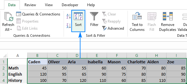
- In the Sort dialog box, click the Options...
- In the small Sort Options dialog that appears, select Sort left to right, and click OK to get back to the Sort
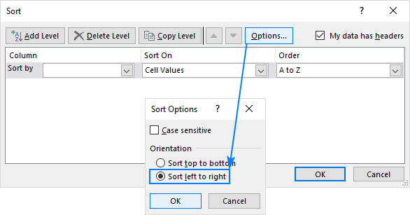
- From the Sort by drop-down list, select the row number you want to alphabetize (Row 1 in this example). In the other two boxes, the default values will do just fine, so we keep them (Cell Values in the Sort on box, and A to Z in the Order box), and click OK:
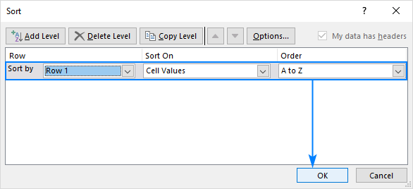
As the result, the first row in our table is sorted in alphabetical order, and the rest of the data is rearranged accordingly, preserving all correlations between the entries:

Problems with sorting alphabetically in Excel
Excel sort features are amazing, but if you are working with an imperfectly structured data, things may go terribly wrong. Here are the two common issues.
Blank or hidden columns and rows
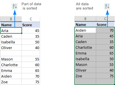
If there are empty or hidden rows and columns within your data, and you select just one cell before clicking the sort button, only the part of your data until the first blank row and/or column will be sorted.
An easy fix is to eliminate the blanks and unhide all hidden areas before sorting. In case of blank rows (not hidden rows!), you can select the entire table first, and then alphabetize.
Unrecognizable column headers
If your column headers are formatted differently from the rest of the data, Excel is smart enough to identify them and exclude from sorting. But if the header row has no special formatting, your column headers will most likely be treated as regular entries and end up somewhere in the middle of the sorted data. To prevent this from happening, select only the data rows, and then sort.
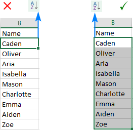
When using the Sort dialog box, make sure the My data has headers checkbox is selected.
How to sort alphabetically in Excel with formulas
Microsoft Excel provides a variety of features to cope with many different tasks. Many, but not all. If you are facing a challenge for which there is no built-in solution, chances are it can be accomplished with a formula. It is also true for alphabetical sorting. Below, you will find a couple of examples when alphabetical order can only be done with formulas.
How to alphabetize in Excel by last name
Since there are a few common ways to write names in English, you may sometimes find yourself in a situation when the entries start with the first name while you need to alphabetize them by the last name:
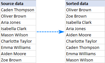
Excel's sort options cannot help in this case, so let's resort to formulas.
With a full name in A2, insert the following formulas in two different cells, and then copy them down the columns until the last cell with data:
In C2, extract the first name:
=LEFT(A2,SEARCH(" ",A2)-1)
In D2, pull the last name:
=RIGHT(A2,LEN(A2)-SEARCH(" ",A2,1))
And then, concatenated the parts in the reverse order separated by comma:
=D2&", "&C2
The detailed explanation of the formulas can be found here, for now let's just focus on the results:
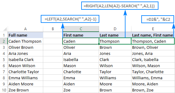
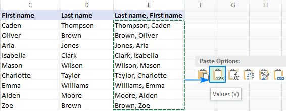
Since we need to alphabetize the names, not formulas, convert them to values. For this, select all the formula cells (E2:E10) and press Ctrl + C to copy them. Right-click the selected cells, click on Values under Paste Options, and press the Enter key:
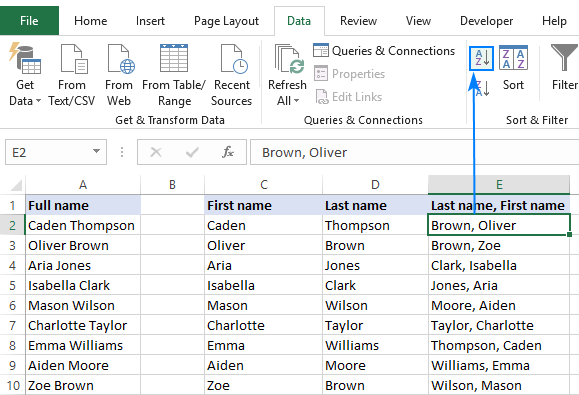
Good, you are almost there! Now, select any cell in the resulting column, click the A to Z or Z to A button on the Data tab, and there you have it - a list alphabetized by the last name:
In case you need to revert to the original First Name Last Name format, there is a little more work for you to do:
Split the names into two parts again by using the below formulas (where E2 is a comma-separated name):
Get the first name:
=RIGHT(E2, LEN(E2) - SEARCH(" ", E2))
Get the last name:
=LEFT(E2, SEARCH(" ", E2) - 2)
And bring the two parts together:
=G2&" "&H2
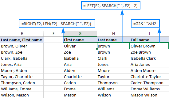
Perform the formulas to values conversion one more time, and you are good to go!
The process may look a bit complex on paper, but trust me, it will take only a few minutes in your Excel. In fact, it will take even less time than reading this tutorial, let alone alphabetizing the names manually :)
How to alphabetize each row individually in Excel
In one of the previous examples we discussed how to alphabetize rows in Excel by using the Sort dialog box. In that example, we were dealing with a correlated set of data. But what if each row contains independent information? How do you alphabetize each row individually?
In case you have a reasonable number of rows, you can sort them one by one performing these steps. If you have hundreds or thousands of rows, that would be an enormous waste of time. Formulas can do the same thing much faster.
Suppose you have many rows of data that should be re-arranged alphabetically like this:

To begin with, copy the row labels to another worksheet or another location in the same sheet, and then use the following array formula to put each row in alphabetical order (where B2:D2 is the first row in the source table):
=INDEX($B2:$D2, MATCH(COLUMNS($B2:B2), COUNTIF($B2:$D2, "<="&$B2:$D2), 0))
Please remember that the correct way to enter an array formula in Excel is by pressing Ctrl + Shift + Enter.

If you are not very comfortable with Excel array formulas, please following these steps to enter it correctly in your worksheet:
- Type the formula in the first cell (G2 in our case), and press Ctrl + Shift + Enter. As you do this, Excel will enclose the formula in {curly braces}. Do not try typing the braces manually, that won't work.
- Select the formula cell (G2) and drag the fill handle rightwards to copy the formula to other cells of the first row (up to cell I2 in this example).
- Select all the formula cells in the first row (G2:I2) and drag the fill handle downwards to copy the formula to other rows.
Important note! The above formula works with a couple of caveats: your source data should not contain empty cells or duplicate values.
If your dataset has some blanks, wrap the formula in the IFERROR function:
=IFERROR(INDEX($B2:$D2,MATCH(COLUMNS($B2:B2),COUNTIF($B2:$D2,"<="&$B2:$D2),0)), "")
Unfortunately, there is no easy solution for duplicates. If you know one, please do share in comments!
How this formula works
The above formula is based on the classic INDEX MATCH combination used to perform horizontal lookup in Excel. But since we need kind of "alphabetical lookup", we have rebuilt it in this way:
COUNTIF($B2:$D2,"<="&$B2:$D2) compares all the values in the same row with each other and returns an array of their relative ranks. For example, in row 2 it returns {2,3,1}, meaning Caden is 2nd, Oliver is 3rd, and Aria is 1st. This way, we get the lookup array for the MATCH function.
COLUMNS($B2:B2) supplies the lookup value. Due to a clever use of absolute and relative references, the returned number is incremented by 1 as we go right. That is, for G2, the lookup value is 1, for H2 - 2, for I2 - 3.
MATCH searches for the lookup value calculated by COLUMNS() in the lookup array returned by COUNTIF(), and returns its relative position. For example, for G2, the lookup value is 1, which is in the 3rd position in the lookup array, so MATCH returns 3.
Finally, INDEX extracts the real value based on its relative position in the row. For G2, it fetches the 3rd value in the range B2:D2, which is Aria.
How to sort each column alphabetically in Excel
If you are dealing with independent subsets of data organized vertically in columns, you can easily tweak the above formula to alphabetize each column individually. Just replace COLUMNS() with ROWS(), make a few column coordinates absolute and row coordinates relative and your formula is ready:
=INDEX(A$3:A$5,MATCH(ROWS(A$3:A3),COUNTIF(A$3:A$5,"<="&A$3:A$5),0))
Please remember it's an array formula, which should be completed with Ctrl + Shift + Enter:

Apart from providing solutions to the tasks that are impossible to accomplished with Excel built-in sort options, formulas have one more (though disputable :) advantage - they make sorting dynamic. With inbuilt features, you will have to resort your data each time new entries are added. With formulas, you can add new data any time and the sorted lists will update automatically.
If you'd rather make your new alphabetical arrangement static, replace formulas with their results by using Paste Special > Values.
To have a closer look at the formulas discussed in this tutorial, you are welcome to download our Excel Alphabetical Order worksheet. I thank you for reading and hope to see you on our blog next week!
 by
by
86 comments
why when i try to sort columns from A-Z it say this can't be done on a multiple range selection
Hi! If I understand your question correctly, the following tutorial should help: Sort by several columns.
Hello
I downloaded my historical data for backtesting a stock trading strategy. This sort feature is great as I have 6 different long and short entries (based on conditions) label long_1 - long_6 and short_1 - short_6. But I am running into an issue.
For each trade, there are 2 rows of data - one row for my entry data and one row for my exit data. The column that contains the long_1 (etc) for the entry then has SL_1 or TP_1 (etc) to demark stop loss or take profit for the exit.
When I import this data - the 2 rows (entry and exit) are right above/below the other.
I am trying to sort the the spreadsheet so that I can view my entries and exits by the specific type of entry. But when I sort the data in that column alphabetically, the entry and exit rows don't stay together - essentially defeating the purpose of sorting them.
Is there a way to link the rows in groups of 2 so that this is possible. For example - there is a header row (= Row 1) but then Row 2 is entry and Row 3 is exit data for the same trade. Row 4 is entry and Row 5 is exit data for the next trade and so on. I would like to line Row 2 and 3, Row 4 and 5, and so on.
Thank you in advance for any and all help!!
Cheers,
MP
Hi! Your related data must be in adjacent columns. Then they will be sorted together. You can split the data into two columns using the Create Cards tool. It is available as a part of our Ultimate Suite for Excel that you can install in a trial mode and check how it works for free.
Ok, thanks!