Today's blog post is all about figuring out the difference between two dates in Google Sheets. You will see lots of DATEDIF formulas to count days, months and years, and learn how NETWORKDAYS is used to count workdays only even if your holidays are based on a custom schedule.
Lots of spreadsheets users find dates confusing, if not extremely difficult, to handle. But believe it or not, there are a few handy and straightforward functions for that purpose. DATEDIF and NETWORKDAYS are a couple of them.
DATEDIF function in Google Sheets
As it happens with functions, their names suggest the action. The same goes for DATEDIF. It must be read as date dif, not dated if, and it stands for date difference. Hence, DATEDIF in Google Sheets calculates the date difference between two dates.
Let's break it down to pieces. The function requires three arguments:
- start_date – a date used as a starting point. It must be one of the following:
- a date itself in double-quotes: "8/13/2020"
- a reference to a cell with a date: A2
- a formula that returns a date: DATE(2020, 8, 13)
- a number that stands for a particular date and that can be interpreted as a date by Google Sheets, e.g. 44056 represents August 13, 2020.
- end_date – a date used as an endpoint. It must be of the same format as the start_date.
- unit – is used to tell the function what difference to return. Here's a full list of units you can use:
- "D" – (short for days) returns the number of days between two dates.
- "M" – (months) the number of full months between two dates.
- "Y" – (years) the number of full years.
- "MD" – (days ignoring months) the number of days after subtracting whole months.
- "YD" – (days ignoring years) the number of days after subtracting whole years.
- "YM" – (months ignoring years) the number of complete months after subtracting full years.
Note. All units must be put to formulas the same way they appear above – in double-quotes.
Now let's piece all these parts together and see how DATEDIF formulas work in Google Sheets.
Calculate days between two dates in Google Sheets
Example 1. Count all days
I have a small table to track some orders. All of them have been shipped in the first half of August – Shipping date – which is going to be my start date. There's also an approximate delivery date – Due date.
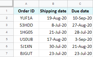
I'm going to calculate days – "D" – between shipping and due dates to see how long it takes for items to arrive. Here is the formula I should use:
=DATEDIF(B2, C2, "D")
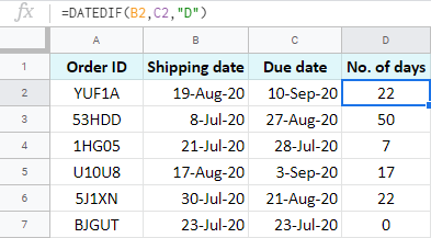
I enter the DATEDIF formula to D2 and then copy it down the column to apply to other rows.
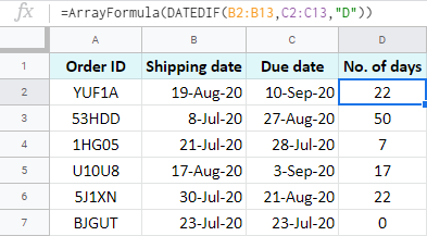
Tip. You can always calculate the entire column at once with a single formula using ARRAYFORMULA:
=ArrayFormula(DATEDIF(B2:B13, C2:C13, "D"))
Example 2. Count days ignoring months
Imagine there are a few months between two dates:
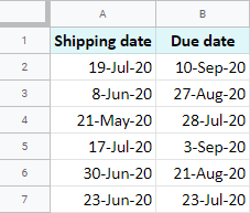
How do you count only days as if they belonged to the same month? That's right: by ignoring full months that have passed. DATEDIF calculates this automatically when you use the "MD" unit:
=DATEDIF(A2, B2, "MD")
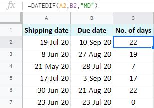
The function subtracts elapsed months and counts remaining days.
Example 3. Count days ignoring years
Another unit – "YD" – will aid for when dates have more than a year between them:
=DATEDIF(A2, B2, "YD")
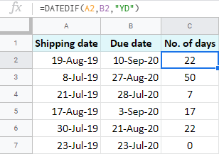
The formula will subtract years first, and then calculate remaining days as if they belonged to the same year.
Count working days in Google Sheets
There is a special case when you need to count only working days in Google Sheets. DATEDIF formulas won't be much of a help here. And I believe you will agree that subtracting weekends manually is not the most elegant option.
Luckily, Google Sheets has a couple of not-so-magic spells for that :)
Example 1. NETWORKDAYS function
The first one is called NETWORKDAYS. This function calculates the number of working days between two dates excluding weekends (Saturday and Sunday) and even holidays if necessary:
- start_date – a date used as a starting point. Required.
Note. If this date is not a holiday, it is counted as a working day.
- end_date – a date used as an endpoint. Required.
Note. If this date is not a holiday, it is counted as a working day.
- holidays – this one is optional for when you need to point out specific holidays. It must be a range of dates or numbers representing dates.
To illustrate how it works, I will add a list of holidays that take place in-between shipping and due dates:

So, column B is my start date, columns C – end date. Dates in column E are the holidays to consider. Here is how the formula should look:
=NETWORKDAYS(B2, C2, $E$2:$E$4)
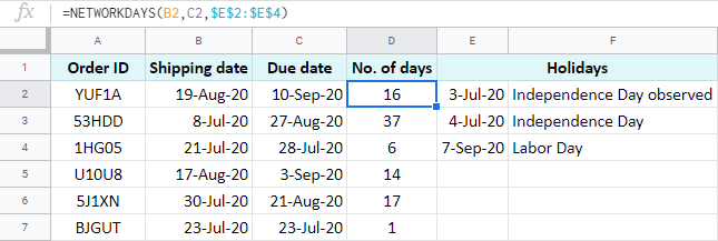
Tip. If you're going to copy the formula to other cells, use absolute cells references for holidays to avoid errors or incorrect results. Or consider building an array formula instead.
Have you noticed how the number of days decreased compared to the DATEDIF formulas? Because now the function automatically subtracts all Saturdays, Sundays, and two holidays that take place on Friday and Monday.
Note. Unlike DATEDIF in Google Sheets, NETWORKDAYS counts start_day and end_day as workdays unless they are holidays. Hence, D7 returns 1.
Example 2. NETWORKDAYS.INTL for Google Sheets
If you have a custom weekend schedule, you will benefit from another function: NETWORKDAYS.INTL. It lets you count working days in Google Sheets based on personally set weekends:
- start_date – a date used as a starting point. Required.
- end_date – a date used as an endpoint. Required.
Note. NETWORKDAYS.INTL in Google Sheets also counts start_day and end_day as workdays unless they are holidays.
- weekend – this one is optional. If omitted, Saturday and Sunday are considered to be weekends. But you can alter that using two ways:
- Masks.
Tip. This way is perfect for when your days off are scattered all over the week.
Mask is a seven-digit pattern of 1's and 0's. 1 stands for a weekend, 0 for a workday. The first digit in the pattern is always Monday, the last one – Sunday.
For example, "1100110" means that you work on Wednesday, Thursday, Friday, and Saturday.
Note. The mask must be put in double-quotes.
- Numbers.
Use one-digit numbers (1-7) that denote a pair of set weekends:
Number Weekend 1 Saturday, Sunday 2 Sunday, Monday 3 Monday, Tuesday 4 Tuesday, Wednesday 5 Wednesday, Thursday 6 Thursday, Friday 7 Friday, Saturday Or work with two-digit numbers (11-17) that denote one day to rest within a week:
Number Weekend day 11 Sunday 12 Monday 13 Tuesday 14 Wednesday 15 Thursday 16 Friday 17 Saturday
- Masks.
- holidays – it is also optional and is used to specify holidays.
This function may seem complicated because of all those numbers, but I encourage you to give it a try.
First, just get a clear understanding of your days off. Let's make it Sunday and Monday. Then, decide on the way to indicate your weekends.
If you go with a mask, it will be like this – 1000001:
=NETWORKDAYS.INTL(B2, C2, "1000001")
But since I have two weekend days in a row, I can use a number from the tables above, 2 in my case:
=NETWORKDAYS.INTL(B2, C2, 2)
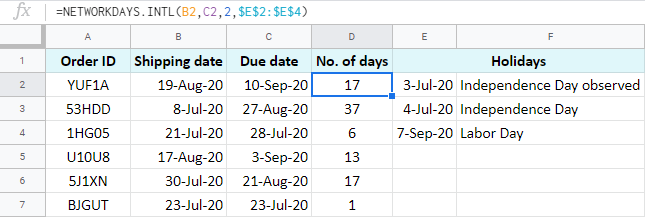
Then simply add the last argument – refer to holidays in column E, and the formula is ready:
=NETWORKDAYS.INTL(B2, C2, 2, $E$2:$E$4)
Google Sheets and date difference in months
Sometimes months matter more than days. If this is true for you and you prefer getting the date difference in months rather than days, let Google Sheets DATEDIF do the job.
Example 1. The number of full months between two dates
The drill is the same: the start_date goes first, followed by the end_date and "M" – that stands for months – as a final argument:
=DATEDIF(A2, B2, "M")
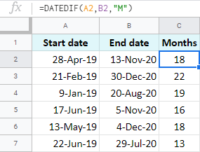
Tip. Don't forget about the ARRAUFORMULA function that can help you count months on all rows at once:
=ARRAYFORMULA(DATEDIF(A2:A13, B2:B13, "M"))
Example 2. The number of months ignoring years
You may not need to count months throughout all years in-between start and end dates. And DATEDIF lets you do that.
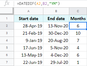
Just use the "YM" unit and the formula will subtract whole years first, and then count the number of months between dates:
=DATEDIF(A2, B2, "YM")
Calculate years between two dates in Google Sheets
The last (but not least) thing to show you is how Google Sheets DATEDIF calculates the date difference in years.
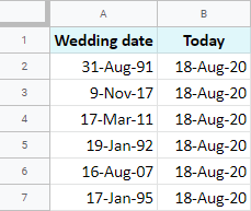
I'm going to calculate the number of years couples have been married based on their wedding dates and today's date:
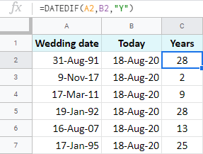
As you may have already guessed, I will use the "Y" unit for that:
=DATEDIF(A2, B2, "Y")
All these DATEDIF formulas are the first to try when it comes to calculating days, months, and years between two dates in Google Sheets.
If your case can't be solved by these or if you have any questions, I encourage you to share them with us in the comments section below.
 by
by
83 comments
hi i would like to ask. if it is possible to calculate a cell with multiple dates. with delimiter " , " if possible the formula i would like to input is datedif.
Hi michael,
You will still need to split the text, even though with a formula. The SPLIT function will help you do that. You can wrap it in other functions and build a longer formula that will split dates and work with the required ones only.
Hi,
For the Data Validation tool in Google Sheets, is there a way or a trick to only select the range that has data instead of the entire column? I like to apply the rule to a specific Data Range (Apply to Range).
Selecting the Column, Data > Data Validation selects the entire Column including the Header, Data and Blank cells in the column. Example: 'Sheet 1'!C1:C2000.
Now I have to manually edit/select the Data Range on the Select the Data Range modal that appears.
Hi Ted,
I'm afraid you have to either select the required range first and then open Data Validation (it will automatically pick up the selected range for 'apply to') or do what you described.
When using the following formula: NETWORKDAYS(C2, D2, Events!B2:B) using the same start-date and end-date such as 1/9/2024 in cell "C2" and 1/9/2024 in cell "D2"
I get a result of 1, but I was expecting a result of 0. What I need to formula to do is calculate the number of days between two dates and excluded dates in a google sheet called "Events" with specific dates listed in cells B2 and below. Any help is most appreciated.
Hello J. Clark,
It's interesting because I'm getting 0 with these dates as an example. For me to be able to help you better, please share an editable copy of your spreadsheet with us (support@apps4gs.com) with (1) a copy of your source data (and the Events sheet) (2) the result you expect to get. I kindly ask you to shorten the tables to 10-20 rows.
Note. We keep that Google account for file sharing only and don't monitor its Inbox. Do not email there. Once you share the file, just confirm by replying to this comment.
I'll look into it and try to help.
Hello Natalia,
I've shared a copy of my Google Sheets with you. Any help is most appreciated.
Thank you for sharing your file!
So apparently I got 0 because I have another date format 😅 My 1/9/2024 is September 1, 2024, which is Sunday. That's why I got 0.
While yours is January 9, 2024, which is Tuesday. If the date is neither holiday nor weekend, it's counted as a working day (I pointed it out in the article). Hence, you've got 1.
Hello Natalia,
What would you recommend using to count days between two dates and get a result of 0 if the dates match? I also need to exclude weekends and holidays or special event dates.
Hello J,
I'd recommend to try and incorporate the IF function: if the dates match, simply subtract 1 to get 0 instead.
I would like to calculate number of days between today and a given future date.
For example between today and 07/02/24.
So every day I open the calcsheet I can se how many days are remaining to the given date
Hello Josef,
You will find formula examples for your case here: Calculate days between two dates in Google Sheets
To have today as a start day, use the TODAY function.
From 8/1/2023 to 10/31/2023, how can I show it's 3 months, instead of 2? Because it we count days, 08/01-08/31, 09/01-09/30, and 10/01 - 10/31 are three whole months.
thanks!
Hi! Remember, the date 10/31/2023 is 10/31/2023 00:00:00. Therefore, that day does not count in the date interval. Your date interval ends on 10/30/2023 23:59:59
Hi! I need to calculate 30 days from 12/1/2023, but if the result day falls on a Saturday or Sunday, I need it to show as the Friday prior. For instance, 30 days from 12/1/2023 is Saturday 12/30/23, I need my spreadsheet to show 12/29/23 instead. How can I do this? Thank you!
Hi Natalia,
You need to use the nested IF function incorporating WEEKDAY in order to check the week day:
=IF(WEEKDAY(A2+B2)=1,(A2+B2)-2,IF(WEEKDAY(A2+B2)=7,(A2+B2)-1,A2+B2))
In this formula, A2 is you start date (12/1/2023) and B2 is the number of days to add.
Hello, very interesting, thankyou.
I have a question slightly off topic. Maybe you could help anyway?
I have a google form where the start date and end date are entered.
What I need is for the response sheet to autopopulate the dates individuelly
So if start date is 06.08.2023 and end date is 08.08.3023 the response sheet input needs to be
06.08.2023
07.08.2023
08.08.2023
I think maybe there isn't a direct way to do this but is it possible at all?
Very gratefull for any help.
Thanks.
Andy.
Hello Andy,
I'm sorry, we don't work with Google Forms and don't know how they record the responses to Sheets.
Hi this is the formula i used to get the age =DATEDIF(J3,TODAY(),"Y")
D.O.B Age today
Jul-04-1994 28
Jan-14-1977 46
Jan-02-1988 35
its not correct its calulating what the age would be this year. what is the formula to calulate number of years and months as at todays date?
Hi Gurbax,
The formula and its results look correct to me.
Jul-04-1994 will be 29 this year. But since it's not July yet, it returns 28. The next two are from January, so they already show this year's age.
Hi.
Can you please help me with formula to add 3 months (Quarterly) in excel.
Example,
14 May 2023
after adding 2 quarter.
14 Nov 2023.
Hi Dibek,
Sorry but this article is about working in Google Sheets. If you need a formula for Excel, please visit this blog post instead since functions work differently in these two platforms: https://www.ablebits.com/office-addins-blog/add-subtract-dates-excel/#add-monts-date
Hi Natalia,
How do I get it to include today as a working day? So for example, start of project was today and it ended by EOD. When I enter 4/21/23 as both start and end date, it results in 0 days. Even though obviously 1 work day was used.
Hi Betty,
Can you please specify the formula you used to count the days?
I have the same question that Betty posed. I would like the data count to be inclusive of the start date and end date. In addition to Betty's example, if I start a task on 5/1 and complete EOD 5/2, it should reveal 2 days. Formula is currently: =DATEDIF(B7,B8,"D"). B7 is start date, B8 is end date.
Hello Jared,
To include the start day in the result, you need to add 1 to your formula:
=DATEDIF(B7,B8,"D")+1
How can I calculate the number days for each month separately when I have a start and finish date that over laps in months. For instance if my star date is 4/15/23and my finish date 5/12/23. How can I get Google sheet to tell me there are 10 business days in April and 10 business days in May? If we can somehow figure out weekend and holidays to be dis-included that would be great.
Hello Juan,
Please see this section to count only working days ignoring weekends and holidays.
But how can I calculate the number days for each month separately when I have a start and finish date that over laps in months. For instance if my star date is 4/15/23and my finish date 5/12/23. How can I get Google sheet to tell me there are 10 business days in April and 10 business days in May?
Thank you for the clarification, Juan.
Here's a formula for April:
=NETWORKDAYS(A2,EOMONTH(A2,0))
And here's for May:
=NETWORKDAYS(EOMONTH(B2,-1),B2)
Hi Natalia,
I would like to calculate resolution time of a certain task based from a given schedule to take out hours of operation including weekends:
Start Date: 3/1/2023 1:16:20
End Date: 3/28/2023 16:00:23
Schedule of Agent during weekdays: 8:00 AM - 5:00 PM
Thanks in advance for the help.
spreadsheet shared
Thank you for sharing the file right away, Candy.
I put the formulas to F & G columns, formatted one as duration and another as days. Please let me know if it helps.
Thanks for your help. Although i see negative computation on my file. Kindly further assist me on this.
Hi Natalia,
Any chance you can help me with the negative #s on my file pls? Same spreadsheet.
Hi Candy,
Yes, sure, I'll look into those negative numbers and reply asap.
Hi Candy,
There's another formula available in your file, please take a look. Sheet Ablebits, column J. I hope this will help you!
I had to create other smaller helper formulas in columns E-I to break down the calculation process. You can hide them or gather everything into one large complex formula.
Thank you so much Natalia.
There are still a few items where it shows negative on my main file when i tried the calculation used on the Applebits sheet. I've added it on that tab as well. Hoping you could check again. Sorry about that.
Hello Candy,
I'll look at your new data and see what I can do.
Hello Candy,
Sorry for the late reply. I'm having difficulties creating one formula for all rows since I don't see a common pattern between them. I have to ask you a few questions:
Can you please provide exact months and days for two difference date like 14 March 2038 with 27 March 2023.
Hello Dibek,
The formulas are provided in these parts of the article:
Calculate days between two dates
Calculate moths between two dates
Hi,
I would like to calculate years and months between two dates, but would like the months to show as a decimal of a year.
So, say A2 is a Start Date of 06-30-2016 (that's MM-DD-YYYY format), and cell B2 is End Date of 12-31-2022. That is 6 years, 6 months. How can I get Google Sheets to show 6.5?
Hi Lorene,
Use this formula:
=YEARFRAC(A2,B2)
Hi Ms. Natalia,
Good day!
How to formulate this, continues the count of days if undelivered from the ATA and stop the count of days if delivered.
I used the below formula but if there is no delivery date, it returns to zero.
=if($H1105="",, MAX(0,DAYS($I1105,MIN(TODAY(),$H1105))))
H = Arrival date at Port
I = Date delivered
I just want to know the number of days that are still at the port and if it stops once delivered.
Many thanks
Hi PedZ Padlan,
Try this formula:
=IF(H2="","",IF(I2="",DAYS(TODAY(),H2),DAYS(I2,H2)))
Hi Ms. Natalia,
Thank you so much
I want to calculate the number of months between today and a date in the past. What formula can I use if I am working on Google Sheets?
Hello Harshit,
You will find the examples in this part of the blog post: Google Sheets and date difference in months
The example that you refer to requires an end date to be specified. What I would like to do is calculate elapsed time between today (which would change depending on when the formula is run) and a date in the past. Showing the number of years, months, days, hours, minutes elapsed. Some start dates are over 365 days ago.
Hello Penny,
DATEDIF is perfectly capable to use today's date, even if it's generated by the TODAY() function.
However, there's no one easy function that would solve your task. You need to use several DATEDIF functions inside CONCATENATE: calculate the date difference of each unit and gather them together into one cell. If time units are necessary as well, the TEXT function will also be a part of your formula (see Example 2 in this article).
Assuming your start date is in A2 and end date is in B2, here's the formula:
=CONCATENATE(DATEDIF(A2,B2,"Y")," years, ",DATEDIF(A2,B2,"YM")," months, ",DATEDIF(A2,B2,"MD")," days, ", TEXT(B2-A2,"h:mm:ss"))
It returns 1 years, 11 months, 30 days, 11:50:00 to a cell.
Hello, maybe someone can help.
if I set a start day (let's say 09 Aug 2022).
In the next column, I set qty of work days = 1
The end date should be calculated automatically (I use WORKDAY formula)
WORKDAY return to me the end date is 10 Aug 2022
But task should be finished in the same date as we started 09 Aug 2022
On the 10 Aug 2022, the next task should be started and the previous task shouldn't be related to 10 Aug 2022
Hello Vadym,
Actually, this is the way the WORKDAY function works. It adds additional working days (1 in your case) to the start date. So there will always be this 1 day jump.
The best way to utilize this function for your task is to set the qty as a number of extra days you'd like to add on top of the first day (0 in your case).
hi. I would like to calculate let say 20 days after the certain date. I am looking to set up a formula. thanks
Hello JES,
Supposing your date is in A2, the following formula will do the trick:
=A2+20
Make sure to format the resulting cell as a Date.
I am receiving different results for the same data range and formula
I have a start and end date that are the same and I am using this formula
=if(S16="","",NETWORKDAYS(J16,S16,Holidays!$B$2:$B$14)-1)
J16 = 1/19/2022
S16 = 1/19/2022
Results in 0
Note: If I remove the -1 at the end, it gives me a 1 but the difference between the dates is 0
I also have the same formula for another date range and its giving me a -1
=if(S17="","",NETWORKDAYS(J17,S17,Holidays!$B$2:$B$14)-1)
J17 = 1/23/2022
S17 = 1/23/2022
Results in -1
Snip of Holiday tab
Holiday Capital One Observed Date
New Year's Day 2022 12/31/2021
Dr. Martin Luther King Jr. Day 1/17/2022
Presidents' Day 2/21/2022
Please help, I can't figure out the discrepancy
Hello Waahida,
Could you please share an editable copy of your spreadsheet with us to support@apps4gs.com
I'll look into it.
Hi Natalia,
I have the same concern, hope you can share the formula. Looking forward to your response.
Hi Leslie,
Undortunately, Waahida has never shared a spreadsheet so I don't really understand the problem.
You can share your file with us as well (support@apps4gs.com), identifying the issue so I know where to look. If you have confidential information there, you can replace it with some irrelevant data, just keep the format. I’ll look into it and try to help.
Note. We keep that Google account for file sharing only and don’t monitor its Inbox. Please do not email there. Once you share the file, just confirm by replying to this comment.
How can calculate the AVG days/months between multiple dates?
Hello Perry,
Have you tried the AVERAGE function? If it doesn't work as you expect, please describe your task in detail and provide examples of your source records and of the expected result.
Hi Natalia,
Hoping to calculate months between two dates but looking for the ability to count half months. so if we start on Oct. 15, 2021 and end on January, 31, 2021, would like to see 3.5 as the calculation result. Any solutions?
Thanks!
Hi Dontae,
You can try something like this to get the more precise fraction results:
=(end_date - start_date)/(365/12)
Question
If I have a networkdays formula that shows me the working days and I want to further break that down to show me working days per each month in the date range that is being calculated what formula would I use ?
Got example if the date range is
July 14,2021 to March 15,2022 and I use network days to figure out the number of working days based on a Monday to Friday
How can I break that’d down further to give me the number of days worked in July,August,sept ,oct etc
Hello Gwen,
The first two arguments of the formula are start_date and end_date. These are the fields where you should indicate the exact periods (months).
I am trying to use DATEDIF to calculate number of months worked . The reference cells for start and end dates are formulas. Even though the formula cells and the input cells are formatted as dates the DATEDIF function returns an error saying they are text....how to resolve this please?
Hi!
I don't know what formulas you are using. They may be using a date but returning text values.
Hello! Which number format does the result cell need to be? I've tried the majority and the output is still 0. Can you help? Thanks!
Hello Lisa,
The Number format should do the trick. If it doesn't work, consider sharing an editable copy of your spreadsheet with us (support@apps4gs.com) and specify the cells to look into. If you have confidential information there, you can replace it with some irrelevant data, just keep the format.
Note. We keep that Google account for file sharing only and don't monitor its Inbox. Please do not email there. Once you share the file, just confirm by replying to this comment.
hello i want to put 2 formulas in one cell e.g
DUEDATE PAID ON
10Jan. 15jan
latefee =(15jan,10jan,”D” now i want to multiplye result with 100 ????
please help
Hello Ankit,
If I get it correctly, a formula like this should help:
=DATEDIF("01/10/2021","01/15/2021","D")*100
Hi Natalia
I am setting up a Google Sheet designed to track project duration, and need a formula to calculate how long a project took to complete.
For example:
Project Start: 30/3/21 at 12:00pm
Project End: 7/4/21 at 5:00pm
I would like a connected cell to autofill with the HOURS taken to complete the project (excluding weekends).
The duration is 148 hours (197- 48)
Assuming Start Date is B2 and End Date is C2, how can I get D2 to calculate the 148 correctly?
This article goes some way to explain the process, but not quite all of it.
Is there a one-line formula that will solve this query?
Thanks
Harvey
Hi Harvey,
Try this formula:
=(NETWORKDAYS(IF(WEEKDAY(B2,2)>5,WORKDAY(B2,1)+1/3,B2),C2)-1+MOD(C2,1)-MOD(IF(WEEKDAY(B2,2)>5,WORKDAY(B2,1)+1/3,B2),1))*24
This worked perfectly. Thank you!
One small glitch - cells to which I've embedded the formula autofill to "-56:00" (negative 56 hours)... But it's not a big issue. Thanks so much.
Harvey,
negative hours may appear if you accidentally change start and end dates places or reference wrong cells. If you'd like, you could share your spreadsheet with us (support@apps4gs.com), we'd look into it as well.
Note. We keep that Google account for file sharing only, please do not email there. Once you share the file, just confirm by replying to this comment.
Hi!
I'd like to calculate how long a task has been pending, so I have a start date, and I want the "end date" to be today, so I can automatically calculate how many months have been spent on a project. Is there a way to use DATEDIF to do that? Thanks!
Hi Spruha,
This part of the blog post explains how to calculate the difference between two dates in months.
If the due date is not in your spreadsheet, you can use the TODAY function in the formula instead of referencing a cell with the due date.
This is very Helpful; thank you. When creating this spreadsheet however, any column without a start date shows that the task has been pending for 44,375 days. How can I have the spreadsheet formatted for future entries to calculate without creating this unusable data?
Hello Chuck,
You can wrap your calculations in the IF function and count only when your start date column contains records.
Thank you!!
My pleasure! :)
Hi
I have invoice date and due date. I can use the formula to calculate the remaining days before due date but how can i stop the calculation or it return as "0" once the column remarks show PAID (manually insert)? Any formula i can combine or do u have some ideas?
Thanks. Appreciate your help
Hi Hirda,
If I understand your task correctly, you can use the IF function to check the status first. If it's something other than 'paid', calculate the number of remaining days. If it's paid, return 0 or something else to your liking.