Learn formulas and formula-free ways to trim whitespaces, remove special symbols (even the first/last N characters) and the same text strings before/after certain chars from multiple cells at once.
Removing the same part of the text from several cells at once can be as important and tricky as adding it. Even if you know some of the ways, you will definitely find new ones in today's blog post. I share plenty of functions and their ready-made formulas and, as always, I save the easiest — formula-free — for last ;)
Formulas for Google Sheets to remove text from cells
I'm going to start with the standard functions for Google Sheets that will remove your text strings and characters from cells. There's no universal function for this, so I will provide different formulas and their combinations for various cases.
Google Sheets: remove whitespace
Whitespace can easily slip into cells after the import or if multiple users edit the sheet at the same time. In fact, extra spaces are so common that Google Sheets has a special Trim tool to remove all whitespaces.
Just select all Google Sheets cells where you want to remove whitespace and choose Data > Trim whitespace in the spreadsheet menu:
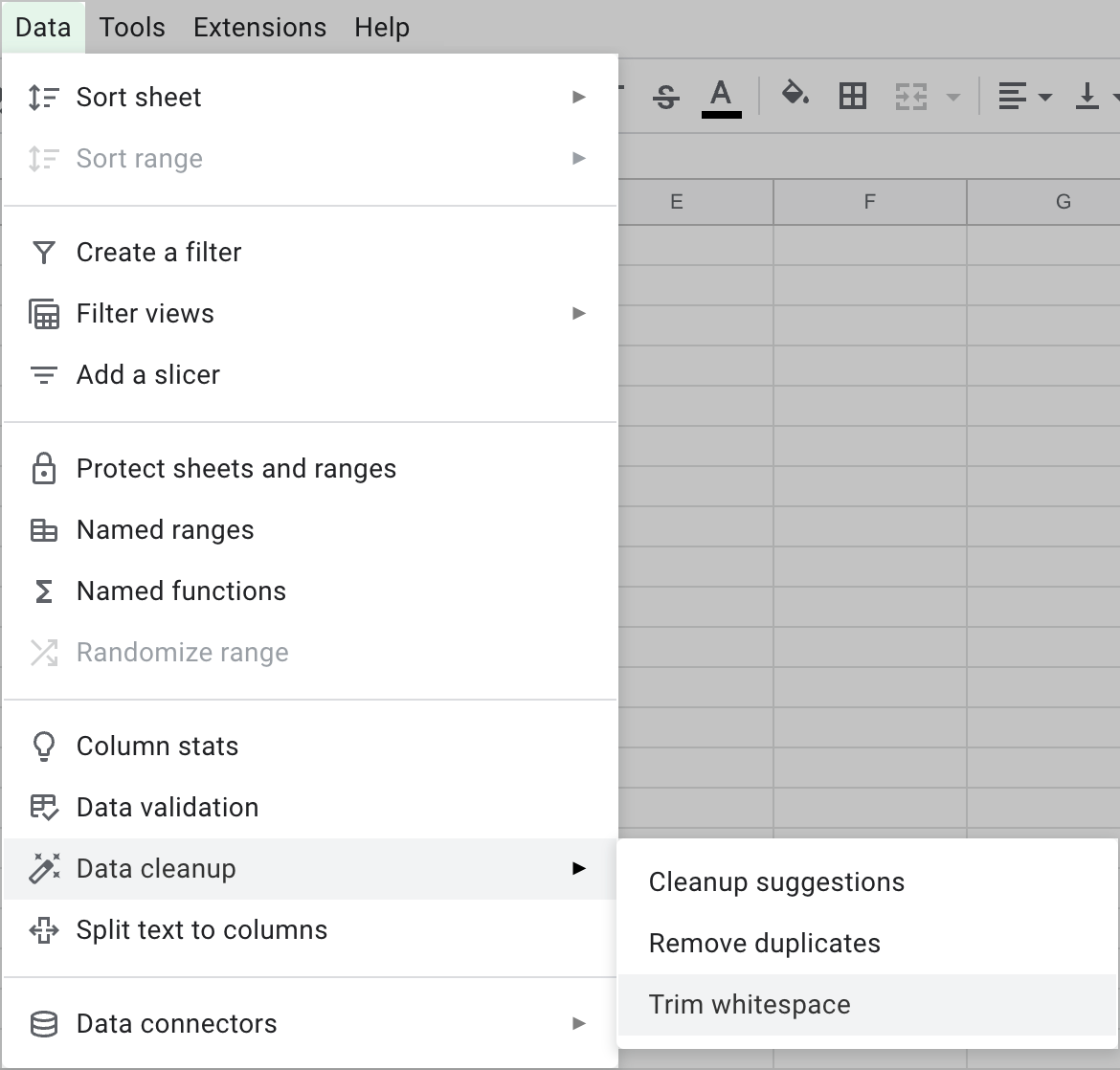
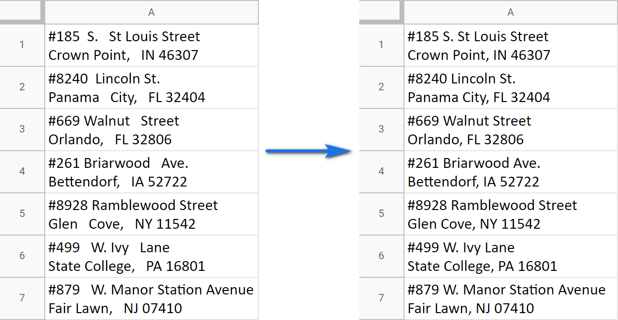
As you click the option, all leading and trailing spaces in the selection will be taken away completely while all extra spaces in-between the data will be reduced to one:
Remove other special characters from text strings in Google Sheets
Alas, Google Sheets doesn't offer a tool to 'trim' other characters but spaces. You have to deal with formulas here.
Tip. Or use our tool instead — Power Tools will free your range from any characters you specify in a click, including whitespace.
Here I have addressed with hashtags before the apartment numbers and phone numbers with dashes and brackets in-between:

I will use formulas to remove those special characters.
The SUBSTITUTE function will help me with that. It is normally used to replace one character with another, but you can turn that to your advantage and replace the unwanted characters with… well, nothing :) In other words, remove it.
Let's see what argument the function requires:
- text_to_search is either the text to process or a cell that contains that text. Required.
- search_for is that character that you want to find and delete. Required.
- replace_with — a character you will insert instead of the unwanted symbol. Required.
- occurrence_number — if there are several instances of the character you're looking for, here you can specify which one to replace. It's completely optional, and if you omit this argument, all instances will be replaced with something new (replace_for).
So let's play. I need to find a hashtag (#) in A1 and replace it with 'nothing' which is marked in spreadsheets with double quotes (""). With all that in mind, I can build the following formula:
=SUBSTITUTE(A1,"#","")
Tip. The hashtag is also in double quotes since this is the way you should mention text strings in Google Sheets formulas.
Then copy this formula down the column if Google Sheets doesn't offer to do that automatically, and you'll get your addresses without the hashtags:
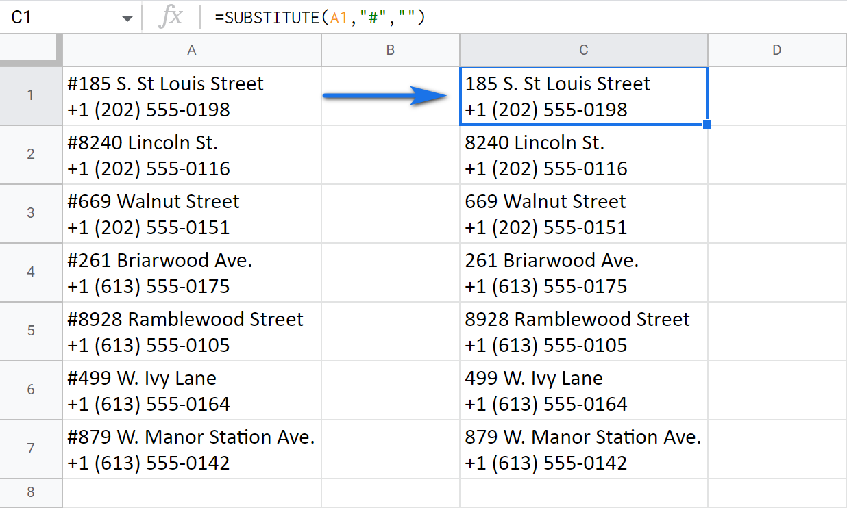
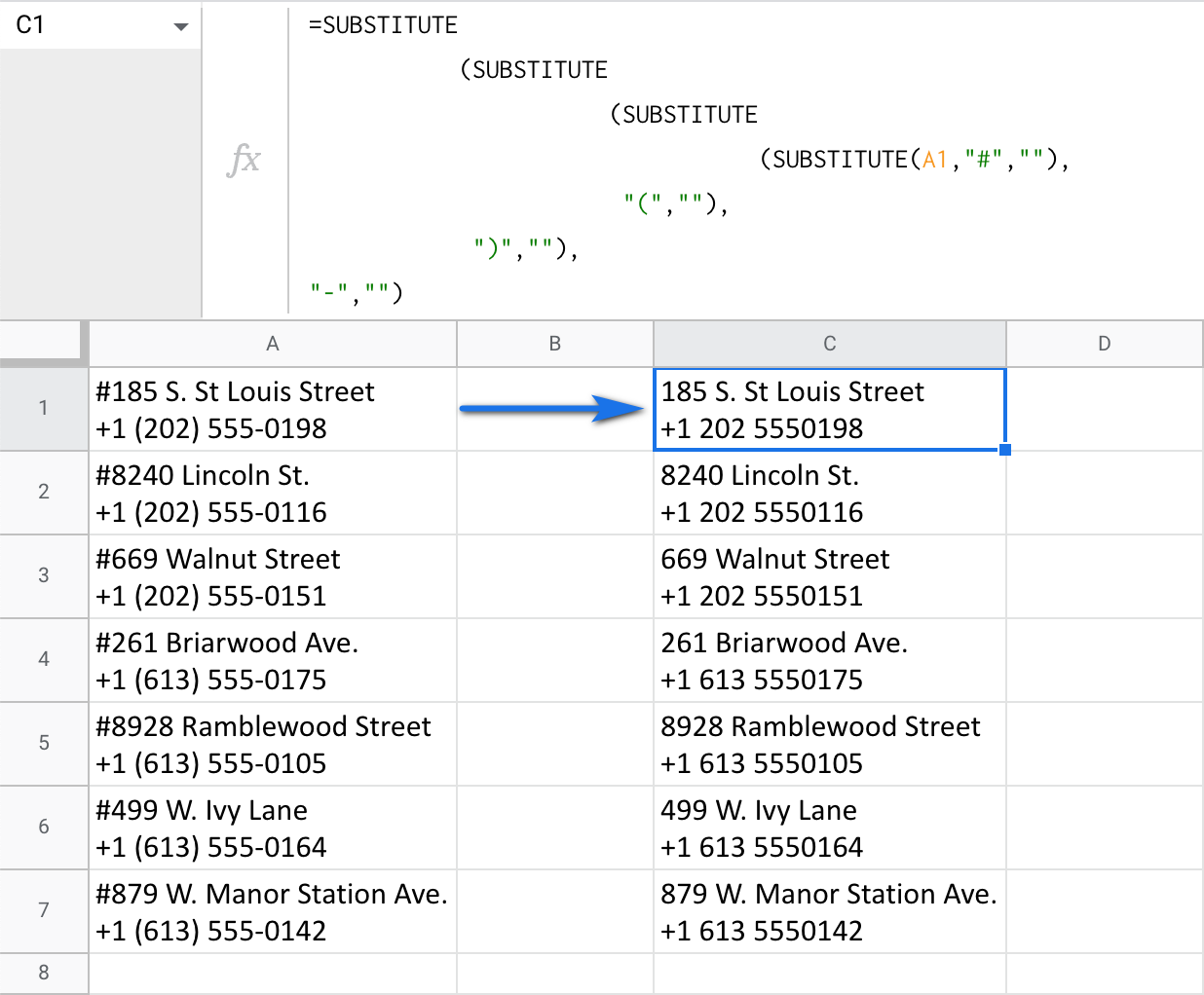
But what about those dashes and brackets? Should you create additional formulas? Not at all! If you nest multiple SUBSTITUTE functions in one Google Sheets formula, you will remove all these characters from each cell:
=SUBSTITUTE(SUBSTITUTE(SUBSTITUTE(SUBSTITUTE(A1,"#",""),"(",""),")",""),"-","")
This formula removes characters one by one and each SUBSTITUTE, starting from the middle, becomes the range to look at for the next SUBSTITUTE:
Tip. What's more, you can wrap this in ArrayFormula and cover the entire column at once. In this case, change the cell reference (A1) to your data in column (A1:A7) as well:
=ArrayFormula(SUBSTITUTE(SUBSTITUTE(SUBSTITUTE(SUBSTITUTE(A1:A7,"#",""),"(",""),")",""),"-",""))
Remove specific text from cells in Google Sheets
Although you can use the aforementioned SUBSTITUTE function for Google Sheets to remove text from cells, I'd like to show another function as well — REGEXREPLACE.
Its name is an acronym from 'regular expression replace'. And I'm going to use the regular expressions to search for the strings to remove and replace them with ' nothing' ("").
Tip. If you're not interested in using regular expressions, I describe a much easier way at the end of this blog post.
Tip. If you're looking for ways to find and remove duplicates in Google Sheets, visit this blog post instead.
As you can see, there are three arguments to the function:
- text — is where you're looking for the text string to remove. It can be the text itself in double quotes or a reference to a cell/range with text.
- regular_expression — your search pattern that consists of various character combinations. You'll be looking for all strings that match this pattern. This argument is where all the fun happens, if I may say so.
- replacement — a new desired text string.
Let's suppose my cells with data also contain the country name (US) if different places in cells:
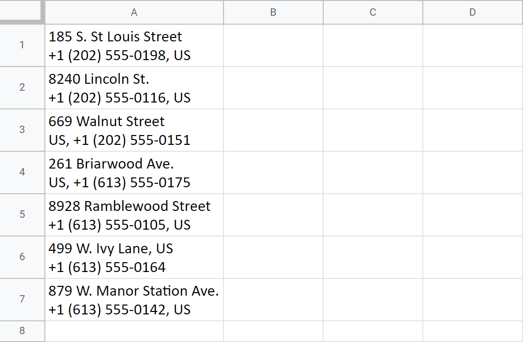
How will REGEXREPLACE help me remove it?
=REGEXREPLACE(A1,"(.*)US(.*)","$1 $2")
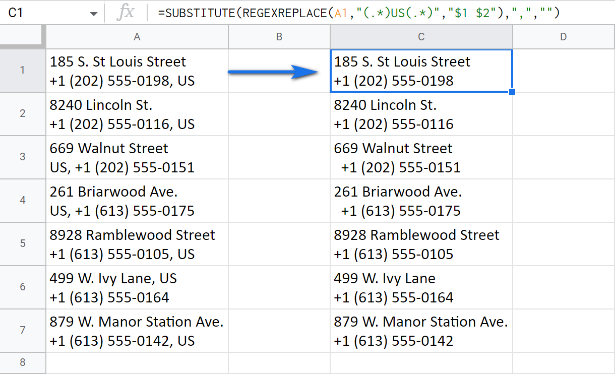
Here's how the formula works exactly:
- it scans the contents of the cell A1
- for matches to this mask: "(.*)US(.*)"
This mask tells the function to look for the US no matter what number of other characters may precede (.*) or follow (.*) the name of the country.
And the entire mask is put to double quotes per the function demands :)
- the last argument — "$1 $2" — is what I want to get instead.$1 and $2 each represent one of those 2 groups of characters — (.*) — from the previous argument. You should mention those groups in the third argument this way so the formula could return everything that possibly stands before and after the US
As for the US itself, I simply don't mention it in the 3rd argument — meaning, I want to return everything from A1 without the US.
Tip. There's a special page you can reference to build various regular expressions and look for the text in different positions of cells.
Tip. As for those remaining commas, the SUBSTITUTE function described above will help to get rid of them ;) You can even enclose REGEXREPLACE with the SUBSTITUTE and solve everything with one formula:
=SUBSTITUTE(REGEXREPLACE(A1,"(.*)US(.*)","$1 $2"),",","")
Remove text before/after certain characters in all selected cells
Example 1. REGEXREPLACE function for Google Sheets
When it comes to getting rid of everything before and after certain characters, REGEXREPLACE also helps. Remember, the function requires 3 arguments:
And, as I mentioned above when I introduced the function, it's the second one you should use correctly so the function knows what to find and remove.
So how do I remove the addresses and keep only phone numbers in cells?
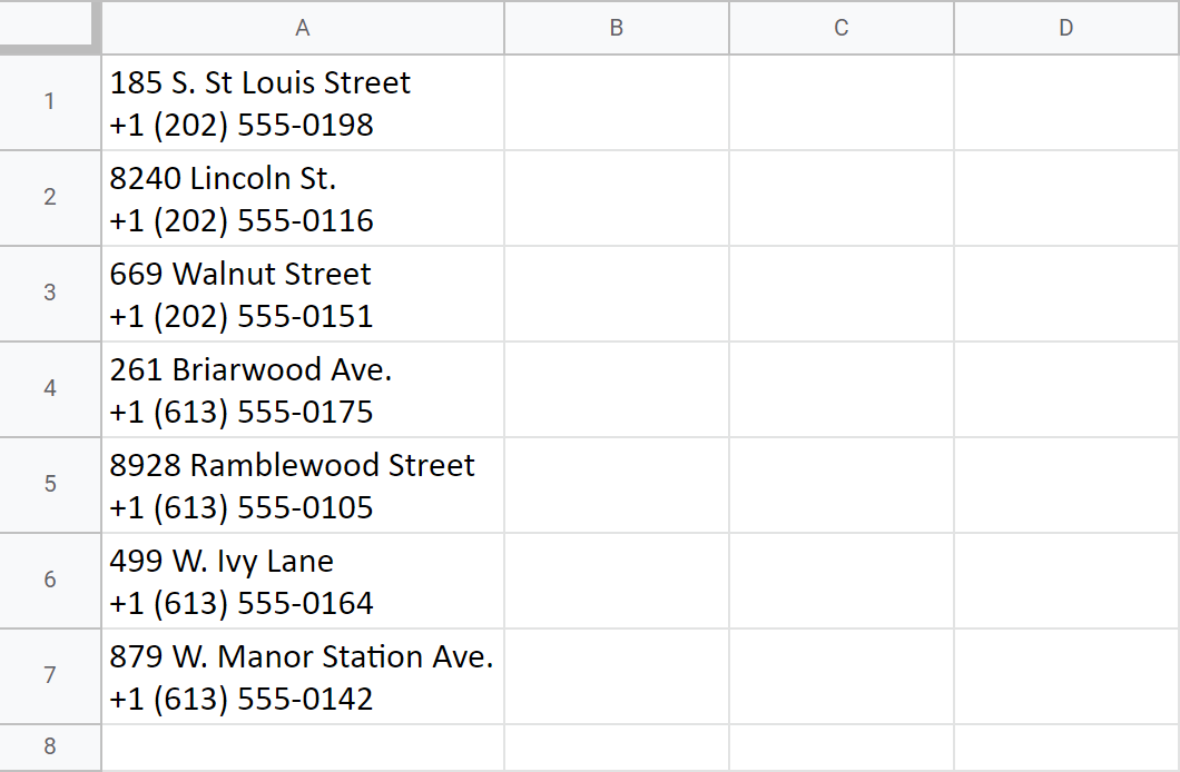
Here's the formula I will use:
=REGEXREPLACE(A1,".*\n.*(\+.*)","$1")
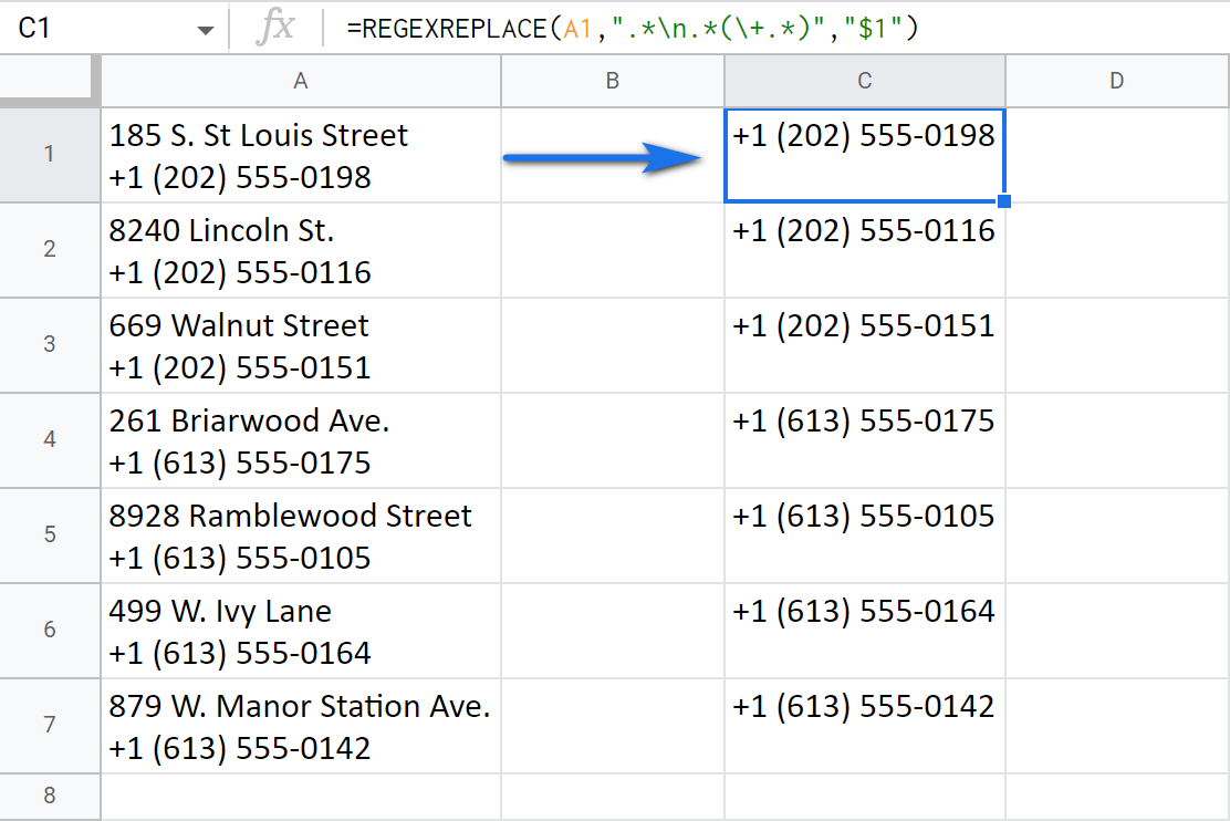
- Here's the regular expression I use in this case: ".*\n.*(\+.*)"
In the first part — .*\n.* — I use backslash+n to tell that my cell has more than one row. So I want the function to remove everything before and after that line break (including it).
The second part that is in brackets (\+.*) says that I want to keep the plus sign and everything that follows it intact. I take this part in brackets to group it and keep it in mind for later.
Tip. The backslash is used before the plus to turn it into a character you're looking for. Without it, the plus would be just a part of the expression that stands for some other characters (as an asterisk does, for example).
- As for the last argument — $1 — it makes the function return that only group from the second argument: the plus sign and everything that follows (\+.*).
Tip. As an alternative, you can simply remove the first line if that'd be easier for your task:
=REGEXREPLACE(A1, "^.*", "")
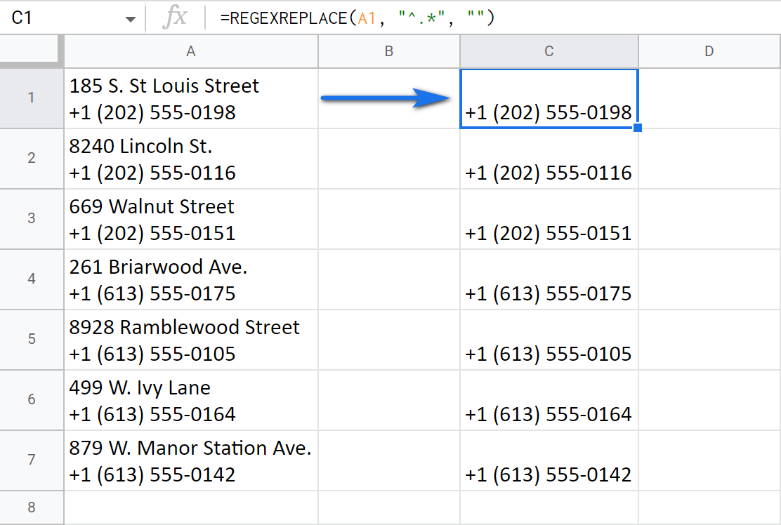
In a similar fashion, you can delete all phone numbers yet keep the addresses:
=REGEXREPLACE(A1,"(.*\n).*","$1")
Only this time, you tell the function to group (and return) everything before the line break and clear out the rest:
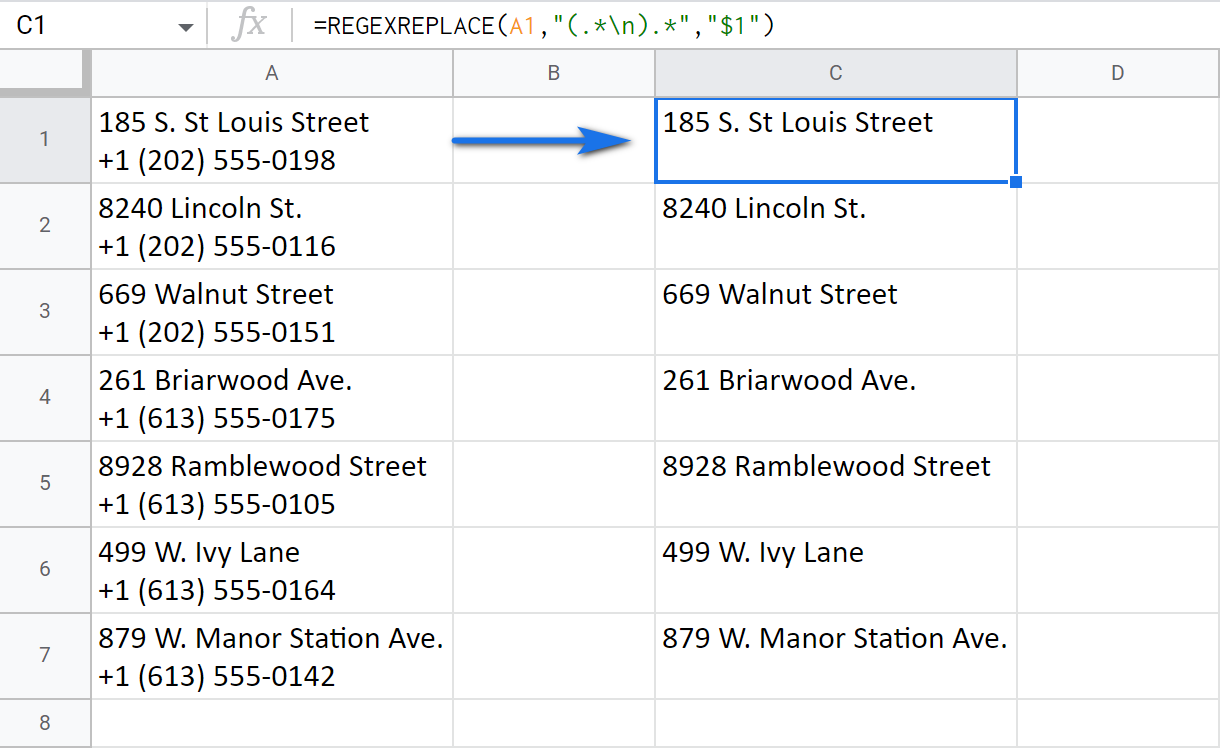
Another case I'd like to mention here concerns the extra info in brackets. Whenever it's irrelevant, there's no point in keeping it in cells. And you have all the means remove to not just everything in-between but also the brackets themselves.
REGEXREPLACE will do that in one go:
=REGEXREPLACE(A1,"\((.*)\)","")
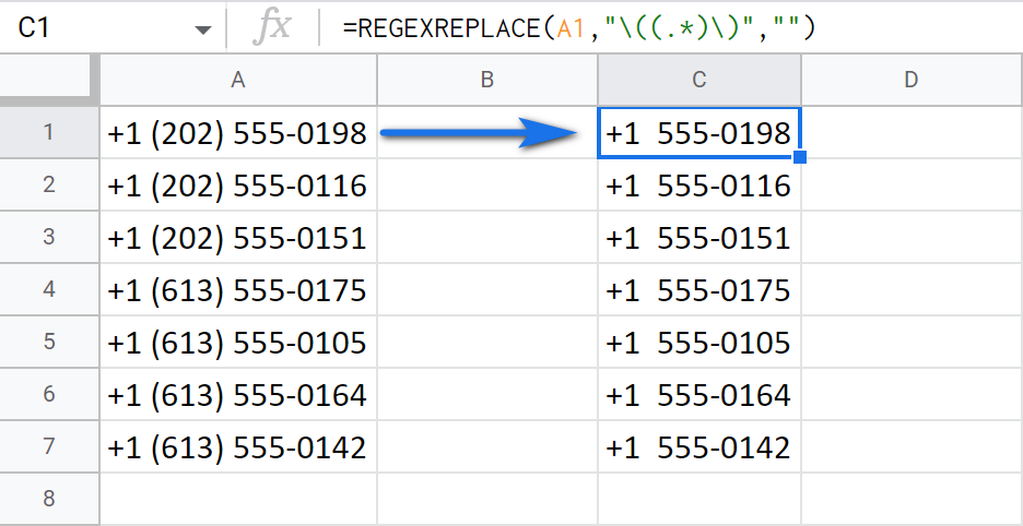
The formula takes:
- the symbol of the opening bracket: \(
- the symbol of the closing one: \)
- and a group of characters between them: (.*)
and replaces them with "nothing" (meaning. removes them): ""
Everything outside them stays intact.
Example 2. RIGHT+LEN+FIND
There are a few more Google Sheets functions that let you remove the text before a certain character. They are RIGHT, LEN and FIND.
Note. These functions will help only if the records to keep are of the same length, like phone numbers in my case. If they're not, just use the REGEXREPLACE instead or, even better, the easier tool described at the end.
Using this trio in a particular order will help me get the same result and remove the entire text before a character — a plus sign:
=RIGHT(A1,(LEN(A1)-(FIND("+",A1)-1)))
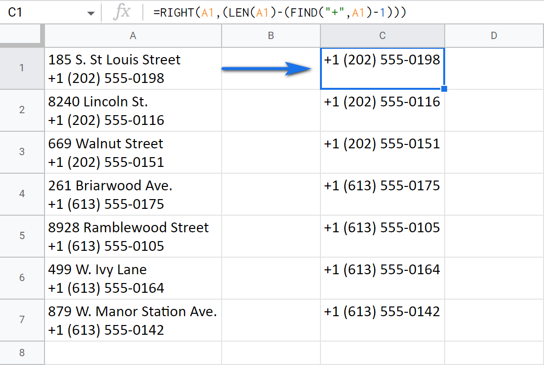
Let me explain how this formula works:
- FIND("+",A1)-1 locates the position number of the plus sign in A1 (24) and subtracts 1 so the total doesn't include the plus itself: 23.
- LEN(A1)-(FIND("+",A1)-1) checks the total number of characters in A1 (40) and subtracts 23 (counted by FIND) from it: 17.
- And then RIGHT returns 17 characters from the end (right) of A1.
Unfortunately, this way won't help much to remove the text after the line break in my case (clear phone numbers and keep addresses), because the addresses are of different length.
Well, that's all right. The tool at the end does this job better anyway ;)
Remove the first/last N characters from strings in Google Sheets
Whenever you need to remove a certain number of different characters from the beginning or the end of a cell, REGEXREPLACE and RIGHT/LEFT+LEN will also help.
Note. Since I already introduced these functions above, I will keep this point short and provide some ready-made formulas. Or feel free to hop to the easiest solution described at the very end.
So, how can I erase the codes from these phone numbers? Or, in other words, remove the first 9 characters from cells:
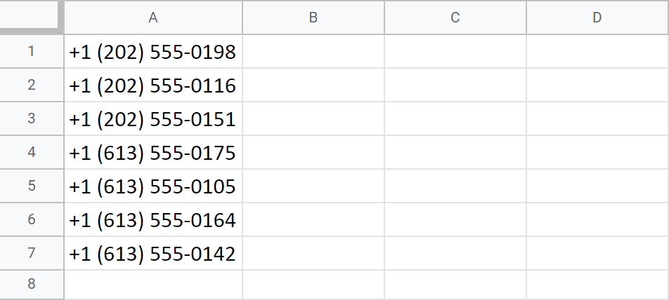
- Use REGEXREPLACE. Create a regular expression that will find and delete everything up to the 9th character (including that 9th character):
=REGEXREPLACE(A1,"(.{9})(.*)","$2")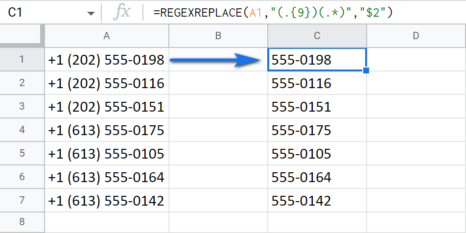
Tip. To remove the last N characters, just swap the groups in the regular expression:
=REGEXREPLACE(A1,"(.*)(.{9})","$1") - RIGHT/LEFT+LEN also count the number of characters to delete and return the remaining part from the end or the beginning of a cell respectively:
=RIGHT(A1,LEN(A1)-9)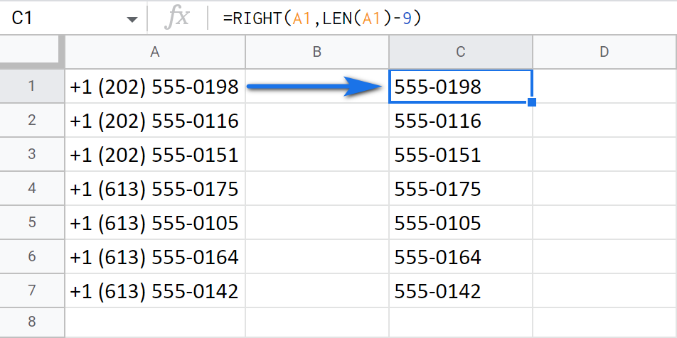
Tip. To remove the last 9 characters from cells, replace RIGHT with LEFT:
=LEFT(A1,LEN(A1)-9) - Last but not least is the REPLACE function. You tell it to take the 9 characters starting from the left and replace them with nothing (""):
=REPLACE(A1,1,9,"")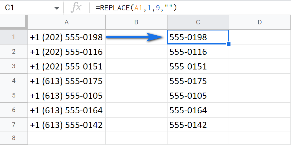
Note. Since REPLACE requires a starting position to process the text, it won't do if you need to delete N characters from the end of a cell.
Formula-free way to remove specific text in Google Sheets — Power Tools add-on
Functions and all is good whenever you have time to kill. But do you know there's a special tool that embraces all of the aforementioned ways and all you are to do is select the required radio button? :) No formulas, no extra columns — you couldn't wish for a better sidekick ;D
You don't have to take my word for it, just install Power Tools and see it for yourself.
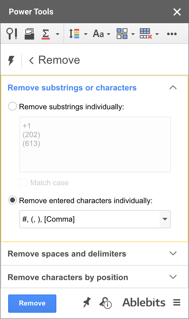
- The first group lets you remove multiple substrings or individual characters from any position in all selected cells at a time:
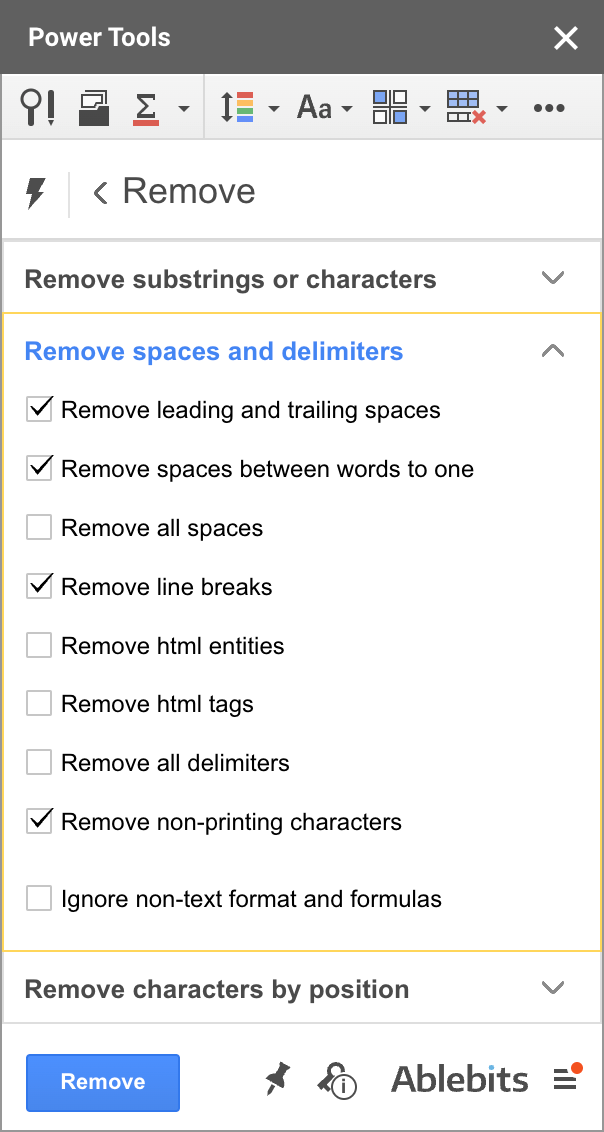
- The next one removes not only spaces but also line breaks, HTML entities & tags, and other delimiters and non-printing characters. Just tick off all the needed checkboxes and press Remove:
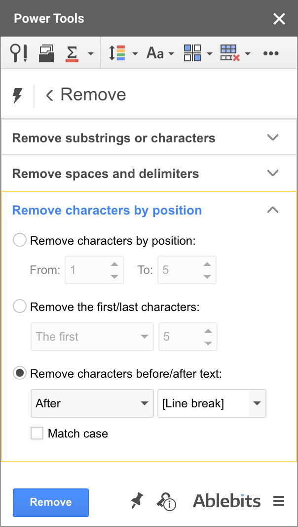
- And finally, there are settings to remove text in Google Sheets by a certain position, first/last N characters, or before/after chars:
Another tool from Power Tools will remove time and date units from timestamps. It's called Split Date & Time:
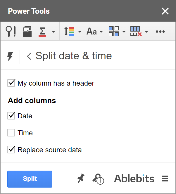
What's the splitting tool got to do with removing time and date units? Well, to remove time from timestamps, select Date since it's a part you want to keep and also tick off Replace source data, just like on the screenshot above.
The tool will extract the date unit and replace the entire timestamp with it. Or, in other words, this add-on for Google Sheets will remove the time unit from the timestamp:
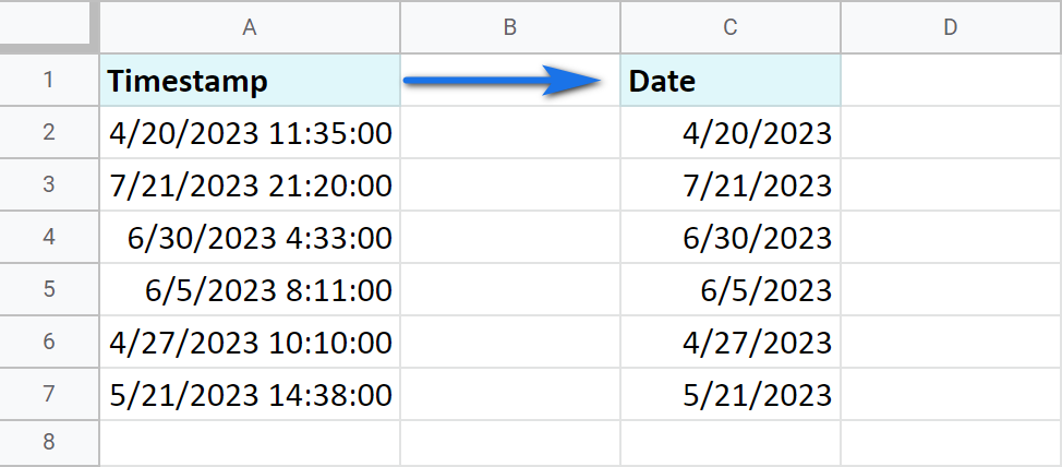
You will have all these and 40+ other time-savers for spreadsheets by installing the add-on from the Google Store.
The first 30 days are completely free and fully functional, so you'll have the time to decide if it's worth any investment.
If you have any questions related to any part of this blog post, I'll see you in the comments section below!
 by
by 
97 comments
Shah, Sonal [9997]
Essig, Chris [175]
Ewalt, Matt [10015]
Quinn, Terry [8613]
example google sheets data, need to remove everything after the name....the find and replace in google sheets will not work for some reason :(. I do not want to create another column.
Hello Lorie,
If you don't want to create another column, use the tool from the last section of the article instead of formulas.
hi,
i have a few datas example as below.
60012345675
60145896646
6001114856001
how do i replace all the data with 6001 in front to 601 without replacing the 6001 at the back of the string?
Really appreciate your help
Hi haslan,
You need to use REGEXREPLACE like in this article. Assuming the number is in A2, this formula will help:
=REGEXREPLACE(TO_TEXT(A2), "^6001", "601")
Feel free to wrap it in ARRAYFORMULA and switch A2 to your entire range of numbers to return the result for all cells at once.
Your examples made using regex so simple.
I am making utility to play wordle. Is there any way to find if a word contails all the letters from string1, say "abcd", but none from string2, say "egfh".
Glad the tutorial is easy, Diba :)
As for your task, assuming the word to check is in A2, try this formula:
=AND(REGEXMATCH(LOWER(A2), "[abcd]"), NOT(REGEXMATCH(LOWER(A2), "[efgh]")))
Thanks Natalia
You're most welcome, Diba!
How can I remove the LAST character of a calculated string?
Please check this part of the article: Remove the first/last N characters from strings in Google Sheets
I am trying to remove the parenthesis () and dash - in a column of phone numbers so it is only a string of numbers.
For example, I am wanting (123) 456-7890 to be replaced with 1234567890.
I have tried several formulas with =REGEXREPLACE but cannot seem to make it work. What would be the proper formula?
Hello Jennifer,
Follow these steps to extract numbers from Google Sheets cells.
Thanks for the info! This was very helpful!
You're most welcome, Luke! Glad the article helped :)
hello ablebits team I did read this great article, but i cant find a way to fix my issue.ıt's easy issue but I want to help me please,
I want to remove before the colon
B8018 : B8018BLK-L2PP
I want this B8018BLK-L2PP
Hello Esma,
I described how to use REGEXREPLACE to remove everything before a character here.
This is the formula that will help you:
=REGEXREPLACE(A2,"(.*)\:(.*)","$2")
I did read this great article, but i cant find a way to fix my issue.
My value in A2 looks like this:
2023-01-01 00:00:01.270976
i need to delete/ replace .270976 how can i do that?
regards
Hello Malosaa,
Since it's a date/time value, you need to solve this via the format – remove milliseconds from it. See the tip at the bottom of this section. The tips from this article may also help you out.
Hello! I got a free template online for a weekly budget tracker.
I need help in removing "$" (US dollar) in some of the cells, and I would like to replace it with a "php" (Philippine peso). The "$" is automatic, and there's nothing in the formula box. Can you help me with this? Thank you so much!
Hello Giana,
That dollar sign appears due to the Currency format applied to cells. To change the currency, select cells and go to Format > Number > Custom currency in the Google Sheets menu, and then pick Philippine Peso.
How do I remove Mr and Mrs from a list of data?
Hello Kira,
You can try one of these methods:
Remove specific text from cells in Google Sheets
Formula-free way to remove specific text in Google Sheets
Hello!
So my manager wants me to clean a sheet for them. Can you help me find a way to just keep the words that contain "#" and then delete everything else on the cell?
Example cell:
#vehiclestatus #rain asdasdasdasd
What I want it to return:
#vehiclestatusi #rain
Is this possible? Thank you.
Hello Wenro,
You need REGEXREPLACE as described in this part of the blog post. Here's how your formula should look:
=REGEXREPLACE(A2," [a-zA-Z]","")
Thank you Natalia! You're amazing!
You're most welcome, Wenro, glad I could help! :)
Hi,
I have a column with some random values: text and numbers.
I want to apply filter formula but the result should contain only text and not numbers. Is there any way around to get this result?
Thanks
Shiv
Hi Shiv,
Try a formula like this:
=FILTER(A2:A10,REGEXMATCH(A2:A10,"[a-zA-Z]")=TRUE)
hello,
How to i remove extra comma(,) from a text Ex- Jhon, Jason, , , , , , , ,. where names are not static and number of characters are not static
Hello Prashanth,
Please specify what this string should like like after removing the required comma. Please also provide a few more examples so I could see what may vary.
Hi,
can you please tell me how to remove "Dracut" with a formula or something in google sheets in the following text:
(1951 Lakeview Ave Dracut)
Hi Ali,
You will find the solution here: Remove specific text from cells in Google Sheets
1951 Lakeview Ave Dracut
=SUBSTITUTE(A2,"Dracut","")
i have assumed that the text is in cell A2
Hi Natalia, appreciate if you could help me... I have the following in each cell:-
World Language
SOC123.1002 4/19
Room SOC1
How do I remove SOC123.1002 only?
Hi Daphne,
Try this formula (assuming your data is in A2):
=REGEXREPLACE(A2, "SOC\d+\.\d+\s+", "")
Sweet, so the thing is that the SOC123.1002 may have a different alphabet depending on the cells, so for example, some would have ENG123.10 and some MAT123.012... can you help to make the formula general so it can apply to all cells?
Sure, here you go:
=REGEXREPLACE(A2, "[A-Z]+\d+\.\d+\s+", "")
YOU are my lfesaver! Thank you so much :)
My pleasure :)
Hi, pls help...
1/4 [5pcs] x 2-1/2
Desired Output: 1/4 x 2-1/2
3/8 [100pcs] x 5
Desired Output: 3/8 x 5
5/16 [fullth] x 1
Desired Output: 5/16 x 1
How to remove the brackets & the chracters inside the bracket?
Hi Jac,
You need to use REGEXREPLACE as described here.
This regular expression will do the job: "(.*) \[.*\](.*)"
I need help with removing everything after a \ in multiple cells. For example, below is what one cell looks like. How would I do that?
Iowa City Comm School District \ Alexander Elementary
Iowa City Comm School District \ Norman Borlaug Elementary School
Non Public \ Faith Academy
Hi Becky,
Assuming this data is in A2, the following formula will do:
=ArrayFormula(JOIN(CHAR(10),REGEXEXTRACT(SPLIT(A2,CHAR(10)),"(.*)\\")))
Hi Natalie!
This post was SO HELPFUL!
I am wondering if you can help me figure something out. I am trying to split the following into three different columns -> *GF Sesame Tofu and Brussels Sprouts* (Vegan, Gluten-Free, Nut-Free, Contains Soy) fried tofu, broccoli, sesame seeds, garlic, ginger, chili house sauce with dry sautéed brussels sprouts and jasmine rice
Column#1: GF Sesame Tofu and Brussel Sprouts [no *]
Column #2: Vegan, Gluten-Free, Nut-Free, Contains Soy [no ()]
Column #3: fried tofu, broccoli, sesame seeds, garlic, ginger, chili house sauce with dry sautéed brussels sprouts and jasmine rice
Please assist! I'm so close. Thank you!
Best,
Katie
Hello!
To extract the text between two characters, use the REGEXEXTRACT function. You can see examples of regular expressions in this article.
=REGEXEXTRACT(A2,"\((.*?)\)")
To extract text after a specific character, use the REGEXEXTRACT function along with the MID function.
=mid(REGEXEXTRACT(A2,"\).*"),2,300)
or
=MID(A2, SEARCH(")", A2)+1, 300)
For more information, please visit: Get text between two characters in Google Sheets.
Thank you SO MUCH! Your solution has saved me!! :D
Hello Natalie,
I am trying to remove every word that appears in a list, I have tried this but it doesn't work =REGEXREPLACE(B2,$C$2:$C$27078,"")
any ideas why?
thanks
Hello Dan,
REGEXREPLACE reqires regular expression as a second argument, while you have a plain range of cells.
Here's what you can try:
Let's say this expression is in A2.
Hope this helps!
Hey Natalia I am trying to use this formula as stated above =REGEXREPLACE(P811,"(.*\n).*","$1") but instead I am trying to delete only the first line rather than everything after the line break. Is that possible?
Hey Brock,
Here you go:
=REGEXREPLACE(P811, "^.*", "")
Hi Natalia is there a way to remove the only first letter of a specific range on sheets?
Hi Mel,
Do you mean the range used in formulas (e.g. turn A2:C10 in formulas to 2:10) or someting else?
Is it possible to use this function to take a cell with existing information (A2) and add the information in another cell (combine A2 and B2) to create a new list, then use it again to take that new list (C2) and remove the information in another cell (D2) to generate a new list?
I tried to add a picture to show it better, but it won't let me. This is a link to a Google Sheet that tries to show it visually: https://docs.google.com/spreadsheets/d/1hlLuvSuBQSV04dxTkyWU9SO1W13sfnEdRVlfCzkONNk/edit#gid=0
Thank you!!!
Hello Julia,
You can merge names from A2 & B2 together using one of the ways from this blog post. The last method is the easiest.
As for removing, you can remove substrings (different names) quickly using our Remove tool as well.
Hi there! So I am trying to create a column where I have a pallet count. I have tried all of the suggested formulas and am still struggling. I have a few examples below. I exported information from a program into excel, but need it for a project I am doing in Google Sheets. I had struggled to create formats and formulas to make this work :(. When I export the information, it appears like below.
I would like to be able to paste this into a google sheets column, with just the beginning number in front of Pallets, and get rid of everything else. Do you have any suggestions?
Thank you!
27Pallets801.58lbs1884.1ft3
1Pallet37.5lbs43.84ft3
Hi Allie,
Try extracting everything before Palett using the way described in this blog post: Extract data before a certain text
Hi!
Is there a way to combine RIGHT and LEFT in one formula cell?
I need to do this...
=LEFT(A1,LEN(A1)-17) and =RIGHT(A1,LEN(A1)-34), all in one cell.
Is there a chance of doing this?
I tried combinen them by brackets, but it doesn't work either
=(RIGHT(A1,LEN(A1)-34)),(LEFT(A1,LEN(A1)-17))
Hi Cynega,
If you need to concatenate both strings returned by LEFT and RIGHT, you can try using one of the methods from this blog post.
Hi Natalia,
I need to delete years and brackets after text e.g DEPARTED, THE (1961). How would I go about doing this so I remain with just DEPARTED, THE
Thank you!
Hi Georgina,
Assuming the data is in A2, try this formula:
=REGEXREPLACE(A2,"(.*)\((.*)","$1")
Hi Natalia
I am a teacher and I create roll lists for house exams. I need to delete names from the lists as the students are sitting there exams in a separate centre.
The software will generate the class list for me but I have to remove names and I have to do this manually.
Is there a formula in Google sheets that I can use where the name is removed. I can easily deal with the empty cell afterwards.
My hope is that if I can use a formula to remove the names, I can then use that formula for various subjects.
Thanks
Kieran
Hi Kieran,
I'm afraid there's no way to remove the contents of a cell by placing a formula there. Formulas return results to the same cells they are used in, and they can't refer to the same cells they are entered in. In this case, you will need to use Apps Script to avoid manual data processing. You may try to find a solution here – an overview of Google Apps Script with a lot of helpful content and links.
Cell data contains:
domainname.comForwards to http: //subdomain.domainname.com
Is there a way to remove everything in a cell from "Forwards to...." to the end?
What I want to end up with is the beginning part:
domainname.com
Thanks
Hello Mario,
Assuming your cell with that record is A2, use this formula:
=REGEXREPLACE(A2,"(.*)Forwards to (.*)","$1")
Look through this part of the article to understand how it works.
This was a very good article. Its explanations were clear and concise. Thank you.
I have a sheet that has phone numbers with a 1 in front of every number. How can I remove it from every number without removing all the 1's in the list? I tried the left, right and len but not getting results.
17137996969
17139565876
12102265350
12107042187
Hello Jack,
Please see this part of the article: How to remove the first N characters
If it still doesn't work, please specify the exact formula you're using.
hey i have data like
$1.5 --in same cell
0.01 -- same cell
$2
0.1
how to split into two column , above method not working
Hey,
Please see this tutorial on how to split cells in Google Sheets into columns.
Is there a way to remove " " ?
For example getting JASON from "JASON"
Thanks !
Hello Jason,
Sure, use this method. The formula will look like this:
=SUBSTITUTE(A2,"""","")
Formula to remove the last period of a sentence in a cell?
Hello Dark,
Please see this section: Remove the first/last N characters from strings in spreadsheets
Thank you, the guide helped a lot...
Question : how would I specificaly delete characters present between any parenthesis and parenthesis themselves ?
like:
Paris (1D4)
London (11)
Berlin (abc)...
Result : "Paris", "London", "Berlin" etc...
Hello Leo,
Try this formula:
=REGEXREPLACE(A1,"(.*)\((.*)\)","$1")
Hi, I would like to delete the text in the cells "K7" when I write " yes " in the cells "L7" do you know how I can do that?
Thanks
Hi Yohan,
Either build the IF formula in any additional cell (to remain empty when 'yes' appears in column L7, otherwise to return the contents of K7) or use Google Apps Script to edit one cell with a record from another.
Is there a way to limit the number of characters that will print out from a column when doing a mail merge. My sheet is to print out spine labels. I have Dewey decimal #, authors last name, and Title. I inputted all data from LibraryThing but I need to limit the Title to maybe the first 20 characters.
Can you think of any way I can do this for the whole column (934 titles).
Thanks so much.
Hello Deborah,
If you'd like to keep all data in cells intact but print out only a limited number of chars, you can simply resize columns before printing the sheet.
If you want to remove chars from cells completely, our Power Tools will help you remove everything after the 20th (or any other) character.
Hi! I just wanted to know how to remove text from a column so its just the numbers when I copy in bank statements.
It looks like:
D
Money In, £, 20.00
Money In, £, 50.00
Money In, £, 15.00
etc
I just want to know how to get rid of the" money in", or how to make the sum without an error.
Hi Lauren,
Based on how your data looks, I'd advise you to look through the last 3 parts of this blog post. You can use any of the ways described there.
Is there a way to mask a list of names due to confidential reasons, which are contained in a column with names? I would like to keep the first name, and mask the second and third words with asterisks, while keeping the first letter of the second and third words.
eg
"Adam John Smith" to "Adam J*** S****
"Charlie Doe" to "Charlie D**"
etc
Many thanks in advance !!!
Hello Calvin,
I'm afraid masks cannot consider the number of characters. So for your case, you can try a formula like this (assuming the data is in A1):
=ArrayFormula(JOIN(" ", ARRAY_CONSTRAIN(SPLIT(A1, " "), 1, 1), REGEXREPLACE(SPLIT(REGEXREPLACE(A1, "^.*?\s+?", ""), " "), "[a-z]", "*")))
Excellent and thanks a lot!
+1 1520-222-9195
+1 1773-443-3769
+1 1480-547-5498
+1 1480-205-2468
+1 1602-339-0394
+1 1480-226-6228
+1 1623-428-4605
+1 1602-921-4482
+1 1928-830-9057
+1 1602-482-9678
+1 1602-330-6397
+1 1602-394-1963
+1 1970-317-1135
+1 1602-371-7951
+1 1623-313-5432
+1 1602-551-5827
Is there a way to remove the number "1" except for those with "+"?
Hello Yusoph,
Yes, if you need to remove those "1" that go right after "+1", you can either try the formulas suggested in this part of the blog post or use the add-on instead, it's much easier and faster.
vm2-01.17
vm2-01.17
vm2-01.17
vm2-01.17
vm2-01.17
vm2-01.17
busy
accepted
vm2-01.17
vm2-01.17
vm2-01.17
vm2-01.17
accepted
busy
I want to remove the ones that contains vm
Hi,
do you want to remove the entire rows or only clear the values from cells?
Hi I have a data set like this.
355
365
957
0563R
043
0576R
754
523
0376R
452
054
0965R
0573R
678
I want to remove 0 value only on the digits end with 'R'. Any specific way to do this without doing each manually. Thanks
Hi there,
Well, you can wrap REGEXREPLACE in ArrayFormula and it will calculate all rows at once. For example, for these 14 rows this formula will do:
=ArrayFormula(IFERROR(REGEXREPLACE(A1:A14,"0(.*)R","$1R"),A1:A14))
Thank you lots. Is there a way to replace/substitute numbers before or after a number or date, eg p5/12/2021 please?
Hello Yohance,
Please give me an example of how your record may look like before and should look after.
I am cleaning up a string which contains *, commas, some other special characters as well as "[9]" in front of name. Every other character was handled except [ ] . While I could introduce an extra substitute function to handle this, is there as way to handle [ ] inside the formula contained in [ ] in one go ?
Hello Nitesh,
Please provide the exact formula you're using so I could suggest a way to improve it.
Hello! I am using a join formula to combine names from one column with the names from another column with an & in-between. For some of the rows, they do not contain a name in the second column so the formula is creating a name followed by an & with nothing following it. Is there a way to remove the &'s that do not have a name following them while leaving the ones that do alone?
Hello Rai,
Try incorporating the IF function for your task. You'll be able to check if the 2nd column contains a name and return a corresponding value.
I appreciate this guide. Is there a way to remove those numbers before or after a person’s name (e.g., Carol20, 123Jason) please?
Hello Dyna,
You can try a formula like this:
=REGEXREPLACE(A2,"[^[:alpha:]]", "")