With this tutorial, you will learn how to find top 3, 5, 10 or n values in a dataset and retrieve matching data.
Want to identify the highest or lowest N values in a column or row? That sounds like a pretty easy thing to do. Need to return not only the values themselves but their names too? Oh, that could be a challenge. There are one or more criteria to be met. Hmm, is that even possible?! Yep, all this can be done with Excel formulas and this tutorial shows how.
Excel formula to find top 3, 5, 10, etc. values
To get the highest N values in a list, use the LARGE and ROWS functions together in this way:
For example, to find top N values in B2:B12, you enter the below formula in the topmost cell where you want the results to appear (D2), and then drag it through as many cells as needed.
=LARGE($B$2:$B$12, ROWS(A$2:A2))
To pull top 3 values, copy the formula to 3 cells.
To get top 5 values, copy the same formula to 5 cells.
To find top 10 values in a column, copy the formula to 10 cells.
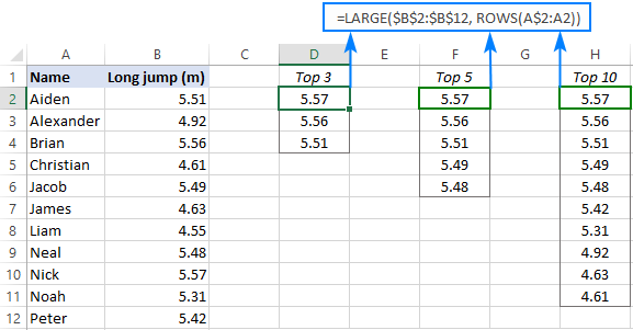
How this formula works:
The LARGE function compares all the numeric values in a range supplied for the 1st argument (array) and returns the largest value based on the position specified in the 2nd argument (k).
The ROWS function with an expanding range reference like ROWS(A$2:A2) generates the k values automatically. To create such a reference, we lock the row coordinate in the first cell with an absolute reference (A$2) and use a relative reference for the last cell (A2).
In the topmost cell where you enter the formula (D2 in this example), ROWS(A$2:A2) generates 1 for k, telling LARGE to return the max value. When copied to the below cells, the range reference expands by 1 row causing the k argument to increment by 1. For example, in D3, the reference changes to A$2:A3. The ROWS function counts the number of rows in A$2:A3 and returns 2 for k, so the LARGE function outputs the 2nd largest value.
Please note that we used A$2:A2 just for convenience because our data begins in row 2. You can use any column letter and any row number for the expanding range reference, say A$1:A1 or C$1:C1.
Excel formula to get bottom 3, 5, 10, etc. values in Excel
To find the lowest N values in a list, the generic formula is:
In this case, we use the SMALL function to extract the k-th smallest value and the ROWS function with an expanding range reference to generate the k number.
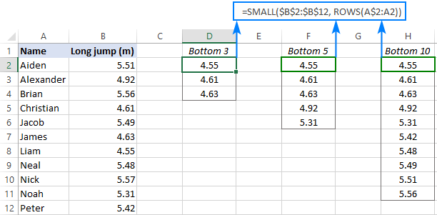
For example, to find bottom N values in the table below, use this formula:
=SMALL($B$2:$B$12, ROWS(A$2:A2))
Enter it in the topmost cell, and then drag down through as many cells as many values you want to get.
Excel formula to find top N values in a row
If your data is organized horizontally in rows, then you can use the following generic formulas to find the highest or lowest values:
Get top values in a row:
Get bottom values in a row:
The formulas' logic is the same as in the previous example with the difference that you use the COLUMNS function rather than ROWS to "feed" the k value to LARGE and SMALL.
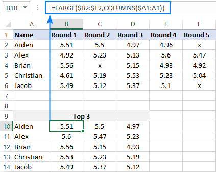
Let's say your table lists the results of 5 rounds for each participant like shown in the image below. You aim to find top 3 values in each row.
To have it done, enter the following formula in the upper-right cell (B10 in our case), and then drag it down and to the right:
=LARGE($B2:$F2, COLUMNS($A1:A1))
For the formula to copy correctly, we use a mixed reference for the array argument of LARGE that locks only the column coordinates ($B2:$F2).
To find bottom 3 values in each row, you can use an analogous SMALL formula:
=SMALL($B$2:$H$2, COLUMNS($A2:A2))
How to get matches of largest N values
In situation when you want to retrieve data relating to top values, use the classic INDEX MATCH formula together with LARGE as the lookup value:
Where:
- Return_array is a range from which to extract associated data (matches).
- Lookup_array is a range where to search for the largest values.
- K is position of the highest value to look for.
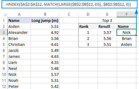
In the table below, you can find top 3 values by using the following approach.
To extract top 3 results, the formula in E3 is:
=LARGE($B$2:$B$12, D3)
Because the ranks are typed in separate cells, the ROWS function is not needed in this case - we simply reference the cell containing the k value (D3).
To retrieve the names, the formula in F3 is:
=INDEX($A$2:$A$12, MATCH(LARGE($B$2:$B$12, D3), $B$2:$B$12, 0))
Where A2:A12 are the names (return_array), B2:B12 are the results (lookup_array) and D3 is the position from largest (k).
In a similar manner, you can get matches of bottom N values. For this, just use the SMALL function instead of LARGE.
To get bottom 3 results, the formula in E3 is:
=SMALL($B$2:$B$12, D3)
To pull the names, the formula in F3 is:
=INDEX($A$2:$A$12, MATCH(SMALL($B$2:$B$12, D3), $B$2:$B$12, 0))
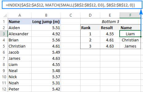
How this formula works:
The LARGE function gets the k-th largest value and passes it to the lookup_value argument of MATCH.
For instance, in F3, we are looking for the 1st largest value, which is 5.57. So, after replacing the LARGE function with its output, the formula reduces to:
=INDEX($A$2:$A$12, MATCH(5.57, $B$2:$B$12, 0))
The MATCH function determines the relative position of 5.57 in B2:B12, which is 9. This number goes to the row_num argument of INDEX, simplifying the formula further:
=INDEX($A$2:$A$10, 9)
Finally, the INDEX function returns the value from the 9th row in the range A2:A12, which is "Nick".
XLOOKUP formula
Microsoft 365 subscribers can achieve the same results by using the new XLOOKUP function:
=XLOOKUP(LARGE($B$2:$B$12, D3), $B$2:$B$12, $A$2:$A$12)
In this case, LARGE returns the k-th largest number directly to XLOOKUP as the lookup value.
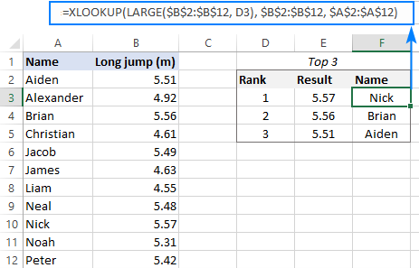
Compared to the INDEX MATCH formula, this syntax is much simpler. However, please keep in mind that XLOOKUP is only available in Excel 365. In Excel 2019, Excel 2016 and earlier versions, this formula won't work.
How to find top values with duplicates
The approach used in the previous example works fine for a dataset that has only unique numbers in the lookup column. Duplicates may lead to wrong results. For example, if the 1st and 2nd largest numbers happen to be the same, the LARGE function will return the same value for each, which is expected by design. But because MATCH returns the position of the first found match, the formula will output the first match twice like shown on the image below:
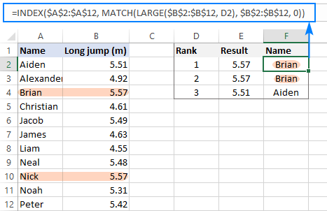
To "break ties" and fix the problem, we need a more sophisticated MATCH function:
=INDEX($A$2:$A$12, MATCH(1, ($B$2:$B$12=LARGE($B$2:$B$12, D2)) * (COUNTIF(F$1:F1, $A$2:$A$12)=0), 0))
In all versions except Excel 365, it only works as an array formula. So, please remember to press Ctrl + Shift + Enter to complete the formula correctly.
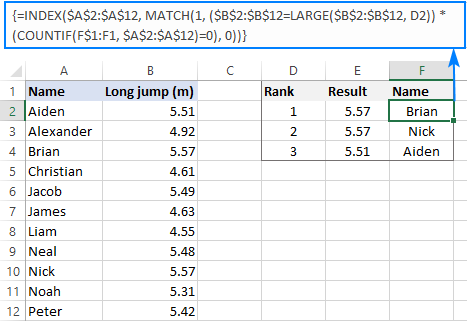
How this formula works:
Here, the MATCH function is configured to search for the number 1, which is the lookup value. The lookup array is constructed using the following logic:
Firstly, all the numbers are compared against the value returned by LARGE:
$B$2:$B$12=LARGE($B$2:$B$12, D2)
Secondly, the COUNTIF function with an expanding range reference checks if a given item is already in the top list. Please pay attention that the expanding range begins on the above row (F1) to avoid a circular reference.
COUNTIF(F$1:F1, $A$2:$A$12)=0
The result of the above operations are two arrays of TRUE and FALSE values, which are multiplied by each other. For example, in F3, we have the following arrays:
{FALSE;FALSE;TRUE;FALSE;FALSE;FALSE;FALSE;FALSE;TRUE;FALSE;FALSE} * {TRUE;TRUE;FALSE;TRUE;TRUE;TRUE;TRUE;TRUE;TRUE;TRUE;TRUE}
In the first array, there are two TRUE values that correspond to 5.57 (rank 1 and 2) - items 3 and 9. But in the second array, item 3 is FALSE because this name (Brian) is already in the list. The multiplication operation changes the logical values TRUE and FALSE into 1 and 0, respectively. And because multiplying by zero always gives zero, only item 9 "survives":
{0;0;0;0;0;0;0;0;1;0;0}
The MATCH function searches for "1" in this array, and returns its relative position (9), which is Nick.
Note. This solution implies that the return column (Name in our case) contains only unique values.
Tip. In Excel 365, you can use a lot simpler FILTER formula that handles ties automatically.
How to find top values in Excel with criteria
To get top values that match certain condition, express your criteria with the help of the IF function and nest them inside the formulas discussed in the previous sections.
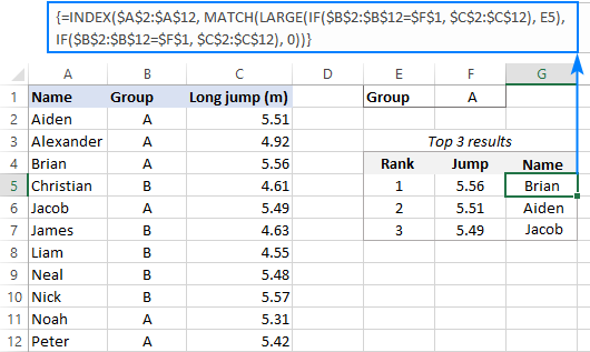
As an example, let's find top 3 results in a given group. To have it done, we input the target group in F1 and type the ranks 1 to 3 in E5:E7 (please see the image below).
To extract top 3 results, enter the below formula in F5 and drag it though F7:
=LARGE(IF($B$2:$B$12=$F$1, $C$2:$C$12), E5)
To ensure that the LARGE function is only processing the results within the target group, we build an IF statement that compares a list of groups against F1.
To get the names, copy this formula in G5 through G7:
=INDEX($A$2:$A$12, MATCH(LARGE(IF($B$2:$B$12=$F$1, $C$2:$C$12), E5), IF($B$2:$B$12=$F$1, $C$2:$C$12), 0))
Here, we use the already familial INDEX MATCH LARGE combination but extend it with two logical tests:
LARGE(IF($B$2:$B$12=$F$1, $C$2:$C$12), E5) - IF checks if a group matches the target one in F1. The matches get into the array from which the LARGE function picks the highest value based on the rank in E5. The result becomes the lookup value for MATCH.
IF($B$2:$B$12=$F$1, $C$2:$C$12) - IF filters out irrelevant groups again, so only the results that belong to the target group make it into the lookup array, where MATCH searches for the lookup value.
These are array formulas that should be entered by pressing Ctrl + Shift + Enter simultaneously. Due to the ability of Excel 365 to handle arrays natively, it's sufficient to press the Enter key in this version.
In Excel 365, you can perform the same logical tests inside XLOOKUP and get the identical results:
=XLOOKUP(LARGE(IF($B$2:$B$12=$F$1, $C$2:$C$12), E5), IF($B$2:$B$12=$F$1, $C$2:$C$12), $A$2:$A$12)
Tips:
- To find bottom values with criteria, simply replace LARGE with SMALL in the above formulas.
- If your dataset contains duplicates, and you want to extract top values and all the names associated with them, here's a working solution for Excel 365: Filter top n values with condition.
- To get top records with multiple criteria, use the FILTER function together with LARGE IF as shown in Filter top n values with multiple criteria.
- In earlier Excel versions, you can extract top/bottom values using advanced filter.
How to FILTER top or bottom values in Excel
In Excel 365, there is a simpler way to find largest N values by using new dynamic array functions such as SORT and FILTER.
Where:
- Data is the source table excluding column headers.
- Numbers are the numeric values to rank.
- N is the number of top entries to extract.
- Sort_index the number of the column to sort by.
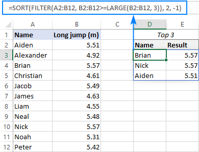
For example, to filter top 3 records in our set of data, the formula goes as follows:
=SORT(FILTER(A2:B12, B2:B12>=LARGE(B2:B12, 3)), 2, -1)
In this case, we set n to 3 because we're extracting top 3 results and sort_index to 2 since the numbers are in the second column.
The beauty of this formula is that you only need to enter it in one cell, and Excel automatically spills the results into as many cells as needed (this concept is called a spill range).
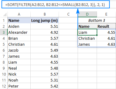
To extract the lowest 3 results, the formula is:
=SORT(FILTER(A2:B12, B2:B12<=SMALL(B2:B12, 3)), 2, 1)
How these formulas work:
Here, we use the FILTER function to filter the source data based on the criteria included in the 2nd argument.
To get top values, we construct the logical expression that checks if a given number is greater than or equal to the Nth highest number in the list (the 3rd largest number in our case): B2:B12>=LARGE(B2:B12, 3).
To get bottom values, we check if a number is less than or equal to the 3rd lowest number: B2:B12<=SMALL(B2:B12, 3).
The result of the logical test is an array of TRUE and FALSE values, which is used for filtering - only the entries corresponding to TRUE get into the final array:
=SORT({"Aiden",5.51;"Brian",5.57;"Nick",5.57}, 2, -1)
As you can see above, the FILTER function outputs the items in the same order they appear in the source range. To sort the results, we place the FILTER formula inside the SORT function and set the sort_order argument to either -1 (descending) or 1 (ascending).
That's how to find top values in Excel. I thank you for reading and look forward to seeing you on our blog next week!
Practice workbook for download
Excel formulas to find top or bottom values (.xlsx file)
 by
by
161 comments
I am trying to get the top n repeated values with criteria and wondering if it's possible with what you have done above. My data has two columns, one is Model Type and the other is Zone.
I need to find the top 3 most repeated values in Zone by Model Type.
Model Type Zone
123 5
123 5
101 4
101 3
123 4
I was able to get the following to work, when I just wanted the top 3 by zone, but now I need to differentiate by Model type as well. Can you help?
= LET(
distinct, UNIQUE(Zone),
count, COUNTIFS(Zone, distinct),
ordered, SORTBY(distinct, count,-1),
INDEX(ordered, {1;2;3}))
Zone =B2:B71
ModelType = A2:A71
Hello! If I understand your question correctly, add another condition to the COUNTIFS function.
= LET(
distinct, UNIQUE(zone),
count, COUNTIFS(zone, distinct,ModelType,$G$1),
ordered, SORTBY(distinct, count,-1),
INDEX(ordered, {1;2;3}))
G1 - model type.
For more information, please visit: Excel COUNTIFS and COUNTIF with multiple criteria.
Hi
Is it possible to pick the top 10 absolute values from a list and then order them by real value so that the positive values are grouped at the top, largest to smallest, followed by the negative values, largest to smallest?
For example:
Currently my top 10 list looks like this:
Entity Value
B 66
C -61
A -53
H -46
F 38
D 33
G -31
S -27
O -23
J 22
I would like the data to look like this:
Entity Value
B 66
F 38
D 33
J 22
C -61
A -53
H -46
G -31
S -27
O -23
Thanks
Hi! There is an inaccuracy in your description. For negative numbers, you are using an ascending sort order. For positive numbers, you use a descending sort order. So you need to use two different sort orders on the data.
By using the FILTER function, we can select the positive numbers and the negative numbers separately.
Then, using the SORT function, we can sort them in the order we want.
These two arrays of values can be combined in a vertical direction by using the VSTACK function.
Based on this information, the formula could be as follows:
=VSTACK(SORT(FILTER(A1:B10,B1:B10>0),2,-1), SORT(FILTER(A1:B10,B1:B10<0),2,1))
Hi I'm trying to find a formula to work out the name of largest value by row by the any individual date of a row I select any ideas?
Hi! If I understand your question correctly, to find the largest value in a row, you can use the examples from the article above. Change the range from column to row in the formulas. If necessary, replace the ROW function with the COLUMN function. If this is not what you wanted, please describe the problem in more detail.
Hi,
I'm trying the "How to find top values with duplicates" but when I enter it, all three of my array formulas are looking for the same Rank (E5 in your example) and returning the same Name. If I change E5 to E6, all the results change to second ranked Name.
my formula is:
=INDEX($A$67:$A$78, MATCH(1, ($B$67:$B$78=LARGE($B$67:$B$78,C80))*(COUNTIF(A$79:A79, $A$67:$A$78)=0), 0))
Names are in A67-A78, Results are in B67-B78, Ranks are in C80-82. I'm looking to return the Top 3 Results in B80-82 & Top 3 Names in A80-82.
Hi! I can't check your formula as I don't have your data. However, note that this formula has no reference to E5. Perhaps you did not enter this formula as an array formula.
Hi,
This has been very helpful! Thank you!!!
I do have a question though.
I have Microsoft 365, so I am able to utilize the SORT FILTER option. I have done this successfully, and it pulls the top 3, and indexes the names associated, which is great. The only problem I am having is that sometimes, one of my top 3 is a zero value, and it pulls all the zero values.
So this is the formula I am using:
=SORT(FILTER(B4:D99,C4:C99>=LARGE(C4:C99,3)),2,-1)
So for example, this would pull
My Top 3 people, their score, frequency of score
Tom, 24,2
Julie, 12,1
Molly, 0,0
Jamie,0,0
Kyle,0,0
etc. until all my zero values have been accounted for.
Is there a way I can modify this formula to exclude all zero values?
Thank you for your time
Hi! If you want to exclude zero values from the results, add another condition to the FILTER function. For example:
=SORT(FILTER(B4:D99,(C4:C99>=LARGE(C4:C99,3))*(C4:C99>0)),2,-1)
For more information, please visit: Excel FILTER function - dynamic filtering with formulas.
This worked like a charm, thank you so much! Hope you have a wonderful day. You have helped me so much!
Hello,
Can you possible do this with a SUMIF or SUMIFS? I have a file that has vendors with multiple categories in a separate column. If I want to sum all the categories for that vendor to find the top vendor, how could I update the formula? Or If I wanted to find the top vendor with category? Thanks!
Hello Michelle! You can use the SUMIFS function to find the amount for each vendor and put it in a specific column. Then use the MAX function to find the maximum value in that column. I also recommend that you read this article: LARGE IF formula in Excel: find highest values with criteria. I hope my advice will help you solve your task.
Many thanks for this article, it has proven very useful. I have been ranking agents on customer feedback scores. Many have scored 100% and the duplicates part of your formula allows me to populate unique names, great! However as part of the ranking I would like to include the number of responses received. This would mean that an agent with 100% from 10 customer feedback forms would rank higher than an agent with 100% from 5 customer feedback forms. Is this possible?
Hi! You can only create a rating for one score. Figure out how to combine your two scores into one overall score and then calculate the rating.
A helpful guide to understanding this thank you. I have SIX columns with a name in row 1, so B1 - Bob, C1 - Joe, D1 - Paul etc. Under each column is a series of numbers and the reference is col A, which for ease of explanation is numbered 1-100 but are irrelevant to this (pretend they are days of work). What I want to do is list the 3 lowest scores for each row in, say, cols J, K and L. So, e.g. row 3, Bob's value is 2.8, Joe is 3.9, Paul is 1.7. On that row in, say, J, K and L I would like Paul in J (lowest), then Bob in K, then Joe in L (just the name, not the values). Row 4 is 5.6, 4.8, 6.2 so J, K and L show Joe, Bob, Paul. Does this make sense? It is so I can see who the three people with the lowest values are out of the six columns with data. Many thanks if you can help.
Hi! The answer to your question can be found in this paragraph of the article above: How to get matches of largest N values.
Here is an example of a formula for a row search:
=INDEX($B$1:$H$1, MATCH(SMALL($B$3:$H$3, 1), $B$3:$H$3, 0))
Thank you, yes I did look at that but I want to return just the name with the lowest and next lowest etc. values (which is over 6 column headers) and not the actual values. I also want them to appear in rows alongside the data. So using 4 rows not 6 as an example:
BOB PETE JOE KEN LOWEST RESULTS HERE
9.94 10.18 8.46 8.88 KEN JOE BOB
9.72 8.88 8.04 9.94 JOE PETE BOB
4.49 4.48 4.73 7.26 PETE BOB JOE
7.07 7.26 7.59 5.7 KEN BOB PETE
Any help appreciated. Thank you.
Why didn't you even try the formula I gave you? It returns the result you want. Change the argument in the SMALL function from 1 to 2 or 3.
Cracked it. I was failing as I didn't have the 1,2,3rd place number in cells, and mine was across rows and not down columns like your example. Thank you so much for your help.
Great tip! I get your function Top value duplicates to work perfectly. Now I just want to add a criteria to the function. How do I do that? I.e. combine "Top values duplicate" with "Top values with criteria"?
I don't want to go with your other example with Filter as it spills out to many cells in my example. And also the values will change frequently.
Hi! The formula Find top values with criteria also shows duplicates. If this is not what you need, please explain in more detail.
Hi
How to display last 10 rows live data in a table
Hi! Add a column of item numbers and use Excel Filter to show "Bottom 10". If this is not what you wanted, describe the problem in more detail.
Hi,
I have a column of n'numbers. I want to display the last 10 numbers in separate table, Is there is way to display like that.
Cheers.
Arun
This is great! However, how do you get rid of duplicates using the last method ("How to find top values in Excel with criteria")? In the example, what happens if two different names have the same long jump result (which is possible)? You can't have Brian show up twice if Aiden also has the same result.
The method "How to find top values with duplicates" does not have a criteria involved.
Hi! Pay attention to the following paragraph: How to FILTER top or bottom values in Excel.
Try this formula:
=SORT(FILTER(FILTER(A2:C12,B2:B12=F1), FILTER(C2:C12,B2:B12=F1)>=LARGE(FILTER(C2:C12,B2:B12=F1), 3)), 2, -1)
Hello,
Hope all is well.
In excel I have 3 columns of data,
Column A: Company
Column B: Return%
Column C: Risk%
Is there a formula I can use to extract only the stocks that have the lowest Risk% with the Highest Return%?
Company Return% Risk%
ABBV 23.76% 5.05%
CVX 16.14% 4.45%
DG 20.91% 4.26%
FDS 20.36% 5.77%
JNJ 17.10% 3.93%
LLY 16.63% 4.99%
LMT 15.05% 5.27%
LOW 18.90% 6.34%
LVMUY 19.00% 6.73%
MA 30.85% 5.15%
MSFT 26.27% 5.69%
NDAQ 15.88% 6.32%
PEP 17.43% 4.09%
PFE 16.24% 4.81%
RTX 14.12% 5.31%
SPY 11.22% 3.50%
T 17.94% 4.64%
V 19.04% 4.38%
VZ 16.00% 4.41%
XOM 15.43% 4.01%
I currently sort the 'Risk%' Column in ascending order, then I scan through the 'Return%' Column to ensure that each subsequent record has a higher Risk% and Return% than the previous record. For example, as shown below I omit: ' XOM 15.43% 4.01%' as with JNJ I get a 17.10% Return% (higher return) for only 3.93% Risk% (lower risk), it doesn't make sense to invest in XOM to receive a lower return% of 15.43% (which is lower than JNJ) and with a higher risk%.
Company Return% Risk%
SPY 11.22% 3.50% - Min Risk% with the Highest Return%
JNJ 17.10% 3.93% - each subsequent record has a higher Risk% and Return% than the previous record.
XOM 15.43% 4.01% DON'T INCLUDE: 15.43% is LESS than the Previous record 17.10%
PEP 17.43% 4.09% - each subsequent record has a higher Risk% and Return% than the previous record.
DG 20.91% 4.26% - each subsequent record has a higher Risk% and Return% than the previous record.
V 19.04% 4.38% DON'T INCLUDE: 19.04% is LESS than the Previous record 20.91%
VZ 16.00% 4.41% DON'T INCLUDE: 16.00% is LESS than the Previous record 20.91%
CVX 16.14% 4.45% DON'T INCLUDE: 16.14% is LESS than the Previous record 20.91%
T 17.94% 4.64% DON'T INCLUDE: 17.94% is LESS than the Previous record 20.91%
PFE 16.24% 4.81% DON'T INCLUDE: 16.24% is LESS than the Previous record 20.91%
LLY 16.63% 4.99% DON'T INCLUDE: 16.63% is LESS than the Previous record 20.91%
ABBV 23.76% 5.05% - each subsequent record has a higher Risk% and Return% than the previous record.
MA 30.85% 5.15% - each subsequent record has a higher Risk% and Return% than the previous record.
LMT 15.05% 5.27% DON'T INCLUDE: 15.05% is LESS than the Previous record 30.85%
RTX 14.12% 5.31% DON'T INCLUDE: 14.12% is LESS than the Previous record 30.85%
MSFT 26.27% 5.69% DON'T INCLUDE: 26.27% is LESS than the Previous record 30.85%
FDS 20.36% 5.77% DON'T INCLUDE: 20.36% is LESS than the Previous record 30.85%
NDAQ 15.88% 6.32% DON'T INCLUDE: 15.88% is LESS than the Previous record 30.85%
LOW 18.90% 6.34% DON'T INCLUDE: 18.90% is LESS than the Previous record 30.85%
LVMUY 19.00% 6.73% DON'T INCLUDE: 19.00% is LESS than the Previous record 30.85%
Here's what the final result should look like:
The Output/ Result should include the Company, Return% and Risk% in Cell E2, F2, & G2
Company Return% Risk%
SPY 11.22% 3.50%
JNJ 17.10% 3.93%
PEP 17.43% 4.09%
DG 20.91% 4.26%
ABBV 23.76% 5.05%
MA 30.85% 5.15%
Hi! Try to enter the following formula in cell D1 and then copy it down along the column:
=--((B1-MAX($B$1:B1))>=0)
The formula returns 0 or 1. Use the Excel filter to select rows with values of 1.
I hope it’ll be helpful.
Hi Alex, great name. For Excel 365 is it possible to use a CSV file that would have 1000 stock symbols (OHLCV) end of day data for 3 years to replace the function of =stockhistory? Meaning the CSV info like a database to then use the formula function for price or volume information?
Hi! I’m sorry, but your task is not entirely clear to me. Could you please describe it in more detail? What result do you want to get? Give an example of the source data and the expected result.
I'll try and explain this as best as I can... I was able to use this formula to get the top 5 highest ratios with names for a weightlifting competition (body weight divided by total weight lifted) but the problem I have is my formula is set to a certain range of cells/rows (for example 1-10) , but if more than 10 competitors enter or less than 10 competitors enter I need to adjust the formula to match the range criteria. Is there any way I can tweak the formula to automatically adjust to the rows filled in (number of competitors)?
This is the formula I used:
=INDEX($C$5:$C$14,MATCH(LARGE($O$5:$O$14,ROWS($Q$5:$Q5)),$O$5:$O$14,0))
Thank you in advance!
Hi!
Your problem can be solved with a dynamic named range. I recommend using this guide: How to create and use dynamic named range in Excel.
This has been so helpful with both pulling top results, and getting rid of my duplicates, but I'm confused about where to put an if statement if I'm also trying to pull the top 3 from different cities (for example).
So if I want the top 3 from City A, City B, and City C but the data is all together, where do I make that work?
Example:
Column A has the cities (cells group named City), B has the stores (cells group named Stores), and C has their results (Cells group named Week1Results)
City A - Store 1 - 50
City C - Store 2 - 99
City C - Store 3 - 15
City B - Store 4 - 44
City A - Store 5 - 22
City A - Store 6 - 50
City B - Store 7 - 20
City C - Store 8 - 30
City A - Store 9 - 12
City B - Store 10 - 36
City B - Store 11 - 50
City C - Store 12 - 30
I had it worked out this way to pull the top ones under the headings of CityA, CityB, etc.: =INDEX(Stores,MATCH(IF(City=CityA,Week1Results),FirstPlace),IF(City=CityA,Week1Results),0))
=INDEX(Stores,MATCH(IF(City=CityB,Week1Results),FirstPlace),IF(City=CityB,Week1Results),0))
And their accompanying results in the next cell: =LARGE(IF(City=CityA,Week1Results),FirstPlace)
=LARGE(IF(City=CityA,Week1Results),SecondPlace)
=LARGE(IF(City=CityA,Week1Results),ThirdPlace)
This worked great until I realised I had the duplicates. On another list where I was just practicing and had only City A stores listed I used the duplicate formula you outlined:
=INDEX(CityAStores, MATCH(1, (CityAWeek1Results=LARGE(CityAWeek1Results,FirstPlace)) * (COUNTIF(F$1:F1, CityAStores)=0),0))
But now I can't figure out how to combine these two and do the duplicate formula while still pulling from the master data list of all the stores with the added criteria of pulling the top 3 from each city. This is obviously simplified, but the data set I'm pulling from has 130 stores across 5 cities with different weeks of results, so just finding this guide has been absolutely amazing.
Hi!
It is very difficult to understand a formula that contains unique references to your workbook worksheets. Hence, I cannot check its work, sorry.