The tutorial shows how to use Advanced Filter in Excel and provides a number of non-trivial criteria range examples to create a case-sensitive filter, find matches and differences between two columns, extract records that match a smaller list, and more.
In our previous article, we discussed different aspects of Excel Advanced Filter and how to use it to filter rows with AND as well as OR logic. Now that you know the basics, let's have a look at more complex criteria range examples that may prove helpful for your work.
Setting up a formula-based criteria range
Since most of the criteria ranges examples discussed in this tutorial are going to include various formulas, let's begin with defining the essential rules to set them up properly. Trust me, this small piece of theory will save you a lot of time and spare the headache of troubleshooting your complex criteria ranges that include multiple conditions based on formulas.
- The formula you use in the criteria range must evaluate to TRUE or FALSE.
- The criteria range should contain at least 2 cells: formula cell and header cell.
- The header cell of the formula-based criteria should be either blank or different from any of the table (list range) headings.
- For the formula to be evaluated for each row in the list range, refer to the top-most cell with data using a relative reference like A1.
- For the formula to be evaluated only for a specific cell or range of cells, refer to that cell or range using an absolute reference like $A$1.
- When referencing the list range in the formula, always use absolute cell references.
- When supplying multiple conditions, enter all of the criteria on the same row to join them with an AND operator, and put each criterion on a separate row to join them with the OR operator.
Excel Advanced Filter criteria range examples
The following examples will teach you how to create your own filters in Excel to handle more complex tasks that cannot be performed using the regular Excel AutoFilter.
Case-sensitive filter for text values
As well as Excel AutoFilter, the Advanced Filter tool is case-insensitive by nature, meaning that it does not distinguish between uppercase and lowercase characters when filtering text values. However, you can easily perform a case-sensitive search by using the EXACT function in the advanced filter criteria.
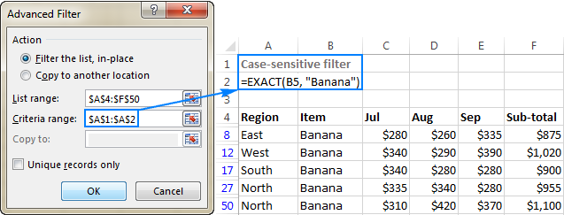
For instance, to filter rows containing Banana, ignoring BANANA and banana, enter the following formula in the criteria range:
=EXACT(B5, "Banana")
Where B is the column containing the item names, and row 5 is the first data row.
And then, apply Excel Advanced Filter by clicking the Advanced button on the Data tab, and configure the List range and Criteria range like shown in the screenshot below. Please pay attention that the Criteria range includes 2 cells - the header cell and the formula cell.
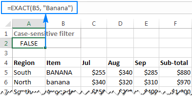
Note. The above image as well all further screenshots in this tutorial show formulas in the criteria range cells solely for the sake of clarity. In your real worksheets, the formula cell should return either TRUE or FALSE, depending on whether the first row of data matches the criteria or not:
Filter values above or below average in a column
When filtering numeric values, you may often want to display only those cells that are above or below an average value in the column. For example:
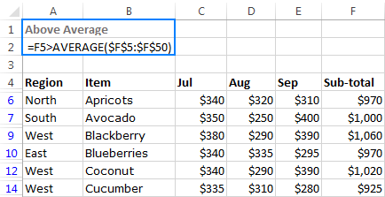
To filter rows with sub-total above average, use the following formula in the criteria range:
=F5>AVERAGE($F$5:$F$50)
To filter rows with sub-total below average, use the following formula:
=F5<AVERAGE($F$5:$F$50)
Please pay attention that we use a relative reference to refer to the top-cell with data (F5), and absolute references to define the entire range for which you want to calculate the average, excluding the column heading ($F$5:$F$50).
The following screenshot demonstrates the above average formula in action:
Those of you who are familiar with Excel Number Filters may wonder, why would someone bother to use an advanced filter while the built-in number filters already have the Above average and Below average options? That's right, but the inbuilt Excel filters cannot be used with the OR logic!
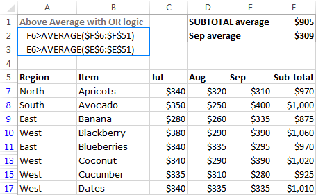
So, to take this example further, let's filter rows where Sub-total (column F) OR September sales (column E) is above average. For this, set up the criteria range with the OR logic by entering each condition on a separate row. As the result, you will get a list of items with the above average values in either column E or F:
Filter rows with blanks or non-blanks
As everyone knows, Excel Filter has an inbuilt option for filtering blank cells. By selecting or deselecting the (Blanks) check box in the AutoFilter menu, you can display only those rows that have empty or non-empty cells in one or more columns. The problem is that the built-in Excel filter for blanks can work only with the AND logic.
If you want to filter blank or non-blank cells with the OR logic, or use the blank / non-blank conditions together with some other criteria, set up an advanced filter criteria range with one of the following formulas:
Filter blanks:
Filter non-blanks:
Filtering blank cells with the OR logic
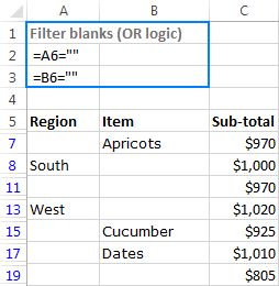
To filter rows that have a blank cell either in column A or B, or in both columns, configure the Advanced Filter criteria range in this way:
=A6=""=B6=""
Where 6 is the top-most row of data.
Filtering non-blank cells with OR as wells as AND logic
To gain more understanding of how Excel's Advanced Filter works with multiple criteria, let's filter rows in our sample table with the following conditions:
- Either Region (column A) or Item (column B) should be non-blank, and
- Sub-total (column C) should be greater than 900.
To put it differently, we want to display rows that meet the following conditions:
(Subtotal>900 AND Region=non-blank) OR (Subtotal>900 AND Item=non-blank)
As you already know, in the Excel Advanced Filter criteria range, the conditions joined with the AND logic should be entered in the same row, and the conditions joined with the OR logic - on different rows:
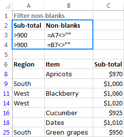
Because one criteria in this example is expressed with a formula (non-blanks) and the other includes a comparison operator (Sub-total > 900), let me remind you that:
- Criteria formed with comparison operators should have headings exactly equal to the table headings, like the Sub-total criteria in the above screenshot.
- Formula-based criteria should have either a blank heading cell or a heading that does not match any of the table headings, like the Non-blanks criteria in the above screenshot.
How to extract top/bottom N records
As you probably know, the build-in Excel Number Filters have an option to display the top 10 or bottom 10 items. But what if you need to filter the top 3 or bottom 5 values? In this case, Excel Advanced Filter with the following formulas comes in handy:
Extract top N items:
Extract bottom N items:
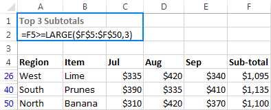
For instance, to filter top 3 subtotals, create the criteria range with this formula:
=F5>=LARGE($F$5:$F$50,3)
To extract bottom 3 subtotals, use this formula:
=F5>=SMALL($F$5:$F$50,3)
Where F5 is the top-most cell with data in the Subtotal column (excluding the column heading).
The following screenshot shows the top 3 formula in action:
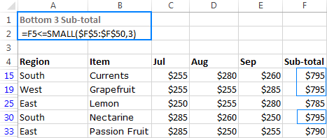
Note. If the list range contains a few rows with the same values that fall into the top/bottom N list, all such rows will be displayed, like shown in the screenshot below:
Filter for matches and differences between two columns
One of our previous articles explained a variety of ways to compare two columns in Excel and find matches and differences between them. In addition to Excel formulas, conditional formatting rules and the Duplicate Remover tool covered in the above tutorial, you can also use Excel's Advanced Filter to extract rows that have the same or different values in two or more columns. To do this, input one of the following simple formulas in the criteria range:
- Filter for matches (duplicates) in 2 columns:
=B5=C5 - Filter for differences (unique values) in 2 columns:
=B5<>C5
Where B5 and C5 are the top-most cells with data in the two columns you want to compare.
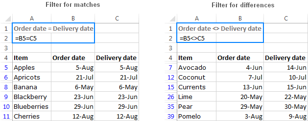
Note. The Advanced Filter tool can only search for matches and differences in the same row. To find all values that are in column A but are not anywhere in column B, use this formula.
Filter rows based on matching items in a list
Supposing you have a big table with hundreds or thousands of rows, and you received a shorter list containing only the items relevant at a given moment. The question is - how do you find all entries in your table that are or are not in the smaller list?
Filter rows that match items in a list
To find all items in the source table that are also present in a smaller list, using the following COUNTIF formula:
Assuming that the smaller list is in the range D2:D7, and the table's items to be compared to that list are in column B beginning with row 10, the formula goes as follows (please notice the use of absolute and relative references):
=COUNTIF($D$2:$D$7,B10)
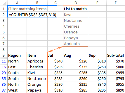
Of course, you are not confined to filtering your table with just one criterion.
For instance, to filter rows matching the list, but for the North region only, enter two criteria in the same row so they will work with the AND logic:
- Region:
="=North" - Matching items:
=COUNTIF($D$2:$D$7,B10)
As you can see in the screenshot below, there are only two records in the table that match both criteria:
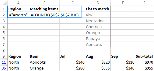
Note. In this example, we use the exact match criteria for text values: ="=North" to find only those cells that are exactly equal to the specified text. If you enter the Region criteria simply as North (without the equal sign and double quotes), Microsoft Excel will find all items that begin with the specified text, e.g. Northeast or Northwest. For more information, please see Excel Advanced Filter for text values.
Filter rows that do not match items in a list
To find all items in the table that are not in the smaller list, check if the result of our COUNTIF formula is equal to zero:
For example, to filter the North region items in the table that do appear in the list, use the following criteria:
- Region:
="=North" - Non-matching items:
=COUNTIF($D$2:$D$7,B10)=0
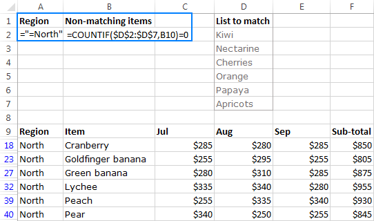
Notes:
- If the list to match resides in a different worksheet, be sure to include the sheet name in the formula, e.g.
=COUNTIF(Sheet2!$A$2:$A$7,B10). - If you want to extract the results to a different sheet, start the Advanced Filter from the destination sheet, as explained in How to extract filtered rows to another worksheet.
Filter for weekends and weekdays
So far, our Advanced Filter criteria range examples have dealt mostly with numeric and text values. Now, it's time to give some clues to those of you who operate on dates.
The built-in Excel Date Filters provide a wide range of options that cover many scenarios. Many, but not all! For example, if you were given a list of dates and asked to filter weekdays and weekends, how would you go about it?
As you probably know, Microsoft Excel provides a special WEEKDAY function that returns the day of the week corresponding to a given date. And it is this function that we are going to use in the Excel Advanced Filter criteria range.
How to filter weekends in Excel
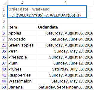
Keeping in mind that, in the WEEKDAY terms, 1 stands for Sunday and 6 stands for Saturday, the formula to filter weekends goes as follows:
In this example, we are filtering dates in column B beginning with row 5, so our Weekends formula takes the following shape:
=OR(WEEKDAY(B5)=7, WEEKDAY(B5)=1)
How to filter weekdays in Excel
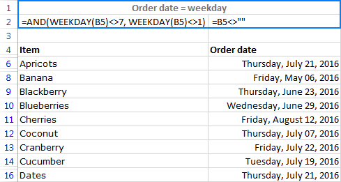
To filter weekdays, modify the above formula so that it will leave out 1's (Sunday) and 7's (Saturday):
For our sample table, the following formula will work a treat:
=AND(WEEKDAY(B5)<>7, WEEKDAY(B5)<>1)
In addition, you can add one more condition to filter out blank cells: =B5<>""
To filter the dates in your worksheets in other ways, just find the relevant Date function and don't hesitate to use it in your advanced filter criteria range.
Well, this is how you use the Advanced Filter in Excel with complex criteria. Of course, your options are not limited to the examples discussed in this tutorial, our goal was just to give you a few inspirational ideas that will set you on the right track. Remembering that the road to mastery is paved with practice, you may want to download our examples using the below link and extend or reverse-engineer them for better understanding. I thank you for reading and hope to see you on our blog next week!
Practice workbook
Excel Advanced Filter examples (.xlsx file)
 by
by
38 comments
While using formula based criteria do we need to compulsorily include heading cell "in the criteria of Advance filter" , i am confused in this, please clear my doubt further in one of the topic "Filter values above or below average in a column" in the 2nd picture the heading cell is ignored, is it by mistake ?
I think its by mistake because in the practice file when ignore taking heading cell i get a different result.
So please clear my doubt.
Thanks
Hello!
The heading cell is not used in advanced filter formulas.
This is an extremely useful piece of information and will make some of my tasks a lot easier, and likely some of my colleagues too.
Regarding this, wondering if there's a way to highlight rows that are new when the content of a cell is changed from "No" to "Yes".
Currently my formula is reading from a different sheet, and giving me the data that I need, based on some conditions.
=FILTER('Sheet'1!$AB$3:$AS$1200,('Sheet1'!$AB$3:$AB$1200="Condition1")*('Sheet1'!$AS$3:AS$1200="Yes"))
Only the values marked as yes on AS will be imported onto the area where the formula is
However, as this can change daily, I need a way to differentiate the previous yes's.
Any idea?
Hello!
If I understand your task correctly, to differentiate previous "yes" add a check condition on the current date.
Greetings! Yes that would be correct!
It's not validated by a specific date however, rather, from changing their "processed" status from "no" to "yes".
Using Advanced Filter how can I filter in place a data table with a date column that will filter out rows that are not between 2 dates that I provide? Thank you
Hello!
Use logical function OR. For example,
=OR(B7<DATE(2016,8,1),B7>DATE(2016,9,1))
Is it possible to use Advanced Filter to filter out rows based on one column of data where any row in that column contains 2 specific items? For example I need to filter out any row in that column that contain both the words MISC and BILLING. I have tried using the advanced criteria range in a couple of different way with no success so far. There are 6 different combinations that it needs to look for to remove that row
MISC and TURN
MISC and CHARGE
MISC and FEE
MISC and DELIVERY
MISC and CUSTOMER
MISC and BILLING
If the advanced filter finds any of these combinations in any row under that column it should filter it out. Thank you for any help you might provide
Hi!
Your explanation is not very clear. To show the cells in which both words are written, create an additional column with a formula like this:
=SUM(--ISNUMBER(SEARCH($D$2:$D$7,B2)))=2
Then set a filter by this column. If this is not what you wanted, please describe the problem in more detail.
Thanks for your comments! I have used the ISNUMBER(SEARCH()) functions before but only for an "OR" condition but not an "AND" condition. You are correct I am trying to show cells in which both words are written. For example both the words "MISC" and "TURN". If I have the following table of words to look for can I use $K$1:$L$8 in your formula above to look for both words?
K L
1 MISC TURN
2 MISC CHARGE
3 MISC FEE
4 MISC DELIVERY
5 MISC CUSTOMER
6 MISC BILLING
7 MISC REBATE
8 MISC DEPOSIT
Hi!
If I got you right, the formula below will help you with your task:
=SUM(ISNUMBER(SEARCH($K$1:$K$8,B2)) * ISNUMBER(SEARCH($L$1:$L$8,B2)))=1
Yes that worked - thank you!
How to get the data using countifs or sumifs from data sheet to another sheet based on multiple (4 or 5 nos.) filter (with dropdown selection which consists of "overall" too) for different months (in columns) ?
Please look into my formula and let me know where it went wrong.
Example:
N1, U1, N3 & U3 - cell reference of dropdown filters
IF(AND($N$1"Overall",$N$3"Overall",$U$1"Overall",$U$3"Overall"),COUNTIFS('Data'!$C:$C,$N$1,'Data'!$H:$H,$U$1,'Data'!$AA:$AA,$N$3,'Data'!$Z:$Z,$U$3),IF(AND($N$3"Overall",$U$1"Overall",$U$3"Overall"),COUNTIFS('Data'!$H:$H,$U$1,'Data'!$AA:$AA,$N$3,'Data'!$Z:$Z,$U$3),IF(AND($N$1"Overall",$U$1"Overall",$U$3"Overall"),COUNTIFS('Data'!$C:$C,$N$1,'Data'!$H:$H,$U$1,'Data'!$Z:$Z,$U$3),IF(AND($N$1"Overall",$N$3"Overall",$U$3"Overall"),COUNTIFS('Data'!$C:$C,$N$1,'Data'!$AA:$AA,$N$3,'Data'!$Z:$Z,$U$3),IF(AND($N$1"Overall",$U$1"Overall",$N$3"Overall"),COUNTIFS('Data'!$C:$C,$N$1,'Data'!$H:$H,$U$1,'Data'!$AA:$AA,$N$3),IF(AND($N$1="Overall",$N$3="Overall",$U$1="Overall",$U$3="Overall"),COUNTIFS('Data'!$AB:$AB,"Overall"),"-"))))))
Hi!
I don't have your workbooks. I can't check the formula that contains unique references to your workbook worksheets, sorry.
Hello!
The drop-down list writes a value to the cell. With the FILTER function, you can filter the values according to this cell.
I hope my advice will help you solve your task.
This is extremely useful. thank you for the very rich and well explained examples.
Create an Advanced Filter using cells A8:K95 as the List range and A1:K2 as the Criteria range. Type the appropriate criterion to only display client records with a total spent amount of more than $6,000.
I WANT TO MAKE A FILTER OR ANY OTHER CODING BY WHICH I CAN FILTER DATA BY INVOICE NUMBER.
I HAVE DATA WHICH HAS INVOICE NUMBER BUT THERE ARE INVOICES WHICH HAS MORE THAN ONE ITEMS AND WHEN I APPLY FILTER IT FILTER ONLY THAT ROW WHICH CONTAIN THE INVOICE NUMBER.
E.G. ROW 1 CONTAIN INVOICE 30 AND COLUMN B HAS ITEMS NOW IF I HAVE 30 IN A1 AND ITEMS IN B1, B2 & B3, NOW I WANT WHEN I APPLY FILTER IT AUTOMATICALLY FILTER ALL ROWS AHICH CONTAIN ITEMS RELATED TO INVOICE 30
Hi !
I have a data set with multiple records per client ID with the client ID repating itself over a couple of rows (its a process flow).
I want to be able filter all the the client IDs where two types of "disposition" (its one of the column) are present.
In other word, some client IDs just have one disposition and some have two. I want my data with just the clien iD that have two.
I figure I can either find a way to excluse the ones that have one or just includes the one that have two but I don't know how.
Thanks for your help,
Sacha
My data comes over from a source that puts the dates into weird format. They look like normal dates, but when i go to format the date this is part of the message on the window that pops up..."...date formats that begin with an asterisk(*) respond to changes in regional date and time settings that are specified for the operating system..."
I called the source people and they said I have to go into my Windows and change the date format there. But when I changed it to the parameters they gave me it messed up everything else on my computer.
Problem is that the Advanced Search doesn't seem to be recognizing them as dates. I've tried the regular 00/00/00 format, as well as a custom format of the same. Any ideas?
My first thought is that of course the people you're getting the data from are not willing to help. Outputting this data as a CSV file would allow you to easily remove the asterisk in Word or another word processor and bring it into Excel.
You should remove the asterisk because Excel displays date and time serial numbers as date values, according to the type and locale (location) that you specify. Date formats that begin with an asterisk (*) respond to changes in regional date and time settings that are specified in Control Panel. Formats without an asterisk are not affected by Control Panel settings. That's what that message means.
I wouldn't mess with the settings in control panel, I'd find a more reasonable workaround.
Have you tired getting the data into Word or another word prosesor, replace the * with nothing and copy and paste that into Excel?
You need to somehow remove the asterisk. Without the asterisk you should be able to put your date and time format back to what you want in Control Panel and then copy the data into Excel and format it as you like in the normal Excel Format Cells window.
I have two columns date and check-in time
Check-in can happen multiple times a day i:e dates column will have duplicate entries .
How to extract all the check-in's for a day ?
Howdy, can anyone help me work this out, but I will likely need some vb to do it. My son has type1 diabetes and uses a continuous glucose monitor, which gets 5 minute blood readings. We callibrate twice a day by a finger prick to make sure the device understands and alters its programming inline with his blood tests. The data I export from the manufacturer shows the word "Calibration" in the row for that time, and I want to select this row if it has that word, then also get the above 12 rows and below 12 rows. The Data example below, you see "EGV" is normal readings it gets each 5 minutes, and when we do a finder prick we add the meters value shown as "Calibration". Future readings should re-adjust its algorithms to be more inline with his blood readings. You see here it was 13 and his finger prick shows 15.6, so the device is out by 2.6, but should then adjust itself to be really close over the future minutes and hours.
In any case i want that calibration row and the 12 above and 12 below it. This will tell me how it has actually changed based on the calibration we enter. As an fyi, these cgms are really close, within 1 number from a blood test, and test the fluid not the blood so is normally 15 minutes behind his blood reading. Sometimes we wait 15-20minutes and see what his cgm gets and its not always the same but is mostly within 1 number out...
timestamp type blood sugar
2017-05-16T19:55 EGV 12.6
2017-05-16T20:00 EGV 12.4
2017-05-16T20:05 EGV 13
2017-05-16T20:07 Calibration 15.6
2017-05-16T20:10 EGV 13.3
2017-05-16T20:15 EGV 15.3
2017-05-16T20:20 EGV 15.2
2017-05-16T20:25 EGV 14.9
I then want to loop all the way down the sheet. I dont think a formula can do it....Thanks, I will keep checking how to do it via formulas but will likely need to write a bit of vb code. Many thanks.
How can I get the subtotal sum value of a data range by removing the duplicated values of a selected criteria
Hi! Can I use advance filter built in excel to exclude from two columns (A & B) all zeroes? Otherwise if filter out in one, in second column not always there is 0, so this makes a mistake. I know formulas can be used, but how's regarding advanced filter? Thanks!
Hello everyone,Challanging question for you all (Please understand the issue carefully before answering hapazardly)
C1:C10 (weight gain)= 1,2,3,4,5,6,7,8,9,10
A1:A10 Age of child in month) = 11,20,23,40,55,60,32,80,90,95,160
Now I make class interval in B1:B10 as (0-1)(2-6)(7-12)(13-24)(25-60)(61-168) for A1:A10
I did: sum age of child meeting (0-1) in B1 which is always showing 0 gram weight increase, for those child who doesnot exist (mistake calculation), want to display empty cell for such case and sum only of there is value in column J. Formulas working fine for the existing child.
I couldnot localize how to calculate for those rows that donot exist in A and display empty cells in B.
Again, for reminder: excel is showing 0 gram increase for those child that doesnot exist in my excel sheet.
I tried 100s of formulas but non of them worked.
Please suggest same formula for all calculating in all class intervals as mentioned above
Please reply this one, not the previous thread
Is there a way to automatically refresh the results if I change the criteria data.
Hi,
I am not sure if I need to use the advance filter or if there is a better way to do this but I could really use your help. I have a table that has a range of zip codes with a minimum and maximum number...ex. State - Alaska Zip Min - 99501 Zip Max - 99950 On my other worksheet I have a large list of customers with zip codes but no states. I would like to add the state column and reference the zip code list and if it falls on or between the min and max number insert the appropriate state. Is this possible? I am not sure where to begin. Thank you!
I am trying to filter a data set using pivot tables but need to only use the top 3 results per participant based on discipline. Please help
Hi, Timothy,
open your pivot table, press filter button, choose Value Filters –> Top 10... You'll see a window, where you'll be able to customize the properties: how many top-results you want to see and according to which criterion. Adjust those to your liking and press OK.
Hi Everyone,
I have an issue or more of a task, I need to build a filter for my data. Everyday I need to send status reports of the shipments made the day prior, but I also need a filter for Mondays, which would include the orders shipped on friday, saturday, and sunday...anyone with any suggestions?
Hi Svetlana
I have a little problem when we transfer on office-2013, especially on excell-2013, precise: I can't find Advanced filter with criteria (criteria is date period of 2, 5, 10, 30 days) in previous excell period I have on cell is like: (>30.09.2016 in cell "A2" and end period is 15.10.2016 in "H2") and formula whose work perfectly but now I can't find these condition, (these condition/dates whose write on cell
Hi,
I am not able to use Advance Filter in which in criteria
True or False.Please find below Details.
Last_Name CFS DCK 90+ Total Login_Hrs. Total
Rashid 120 71 84 275 123.2431402 TRUE
kumar 45 46 86 177 47.48628049
Chaudhary 23 52 87 162 25.68597561
Kumar 124 46 81 251 126.4253049
Kushwaha 46 56 85 187 48.78658537
Verma 120 71 84 275 123.2431402
Singh1 98 63 89 250 101.0541159
Subhani 126 53 83 262 128.6684451
kumar 125 30 120 275 127.4009146
Hello everyone,Challanging question for you all (Please understand the issue carefully before answering hapazardly)
C1:C10 (weight gain)= 1,2,3,4,5,6,7,8,9,10
A1:A10 Age of child in month) = 11,20,23,40,55,60,32,80,90,95,160
Now I make class interval for B1:B10 as (0-1)(2-6)(7-12)(13-24)(25-60)(61-168) in F1:F6
I did: sum age of child meeting (0-1) in B1 which is always showing 0 gram weight increase, for those child who doesnot exist (mistake calculation), want to display empty cell for such case and sum only of there is value in column J. Formulas working fine for the existing child.
I couldnot localize how to calculate for those rows that donot exist in J and display empty cells in F.
Again, for reminder: excel is showing 0 gram increase for those child that doesnot exist in my excel sheet.
I tried 100s of formulas but non of them worked.
Please suggest same formula for all calculating in all class intervals as mentioned above
Hi Svetlana,
How can I used Excel 'Advanced Filter' to filter out those rows that contains certain keywords that met multiple criteria?
Below is the example:
A B
1 00 MAG,NET,PIN,POT
2 01 NET,OIL,RIZ,SAW
3 02 TAP,WAX,YAM,ZIP
For instance, I want Excel Advanced Filter to help me filter out those row that contains either OIL or SAW or YAM. How can I achieve this?
Please advice.
Thank you.
Brian
Hi Svetlana
I have a complicated excel problem and need your help please. It is too long for this space, so I can send you via email once you have replied. That way i can get your email address
Take Care
Willie
Hi Willie,
You can post the details of your problem on our forum, and we will do our best to help you.