This tutorial introduces 2 new functions from our Function by Color add-on for Google Sheets: CELLCOLOR & VALUESBYCOLORALL. Use them to sum & count cells not only by their colors but also by the common contents. Ready-made IF, SUMIFS & COUNTIFS formulas are included ;)
If you work with colored cells in Google Sheets a lot, you may have probably tried our Function by Color add-on. Little do you know that now there are 2 more functions: CELLCOLOR and VALUESBYCOLORALL. They expand your operations with colored cells even further. In this tutorial, I will show you how both functions work and share some ready-made custom formulas.
How to sum and count colored cells in Google Sheets
Before we dive into our 2 new custom functions, I'd like to briefly describe our Function by Color add-on in case you're not familiar with it.
This add-on for Google Sheets checks font and/or fill colors in the selected cells and:
- sums numbers with a common hue
- count cells by color (even blanks)
- finds the average/min/max values among those highlighted cells
- and more
In total, you can use 13 functions to calculate your colored cells.
Here's how it works:
- You select the range to process.
- Select the font and/or fill hues you want to consider and pick the function according to your task.
- Choose to calculate records in each row/column or entire range.
- Select cell(s) where you want to see the result.
- Hit Insert function.
For example, in this Google Sheets table, I sum by color all those items that are 'on their way' (blue color):
=SUM(VALUESBYCOLOR("light cornflower blue 3", "", B2:E2))
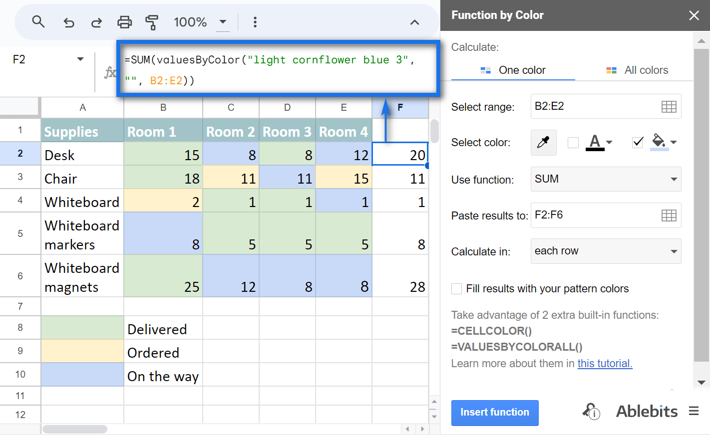
Tip. There's a detailed tutorial for the add-on available here and a blog post with examples here.
As you can see, the add-on uses the standard SUM function along with a special function inside: VALUESBYCOLOR.
VALUESBYCOLOR function
VALUESBYCOLOR is our custom function.
Note. You won't find it in spreadsheets without the add-on.
It returns those cells that correspond to the colors you select in the add-on:
=VALUESBYCOLOR("light cornflower blue 3", "", B2:E2)

See? It gets only those numbers for each item from above that have a fill color from my settings. And it uses one of the standard functions that you select in the tool to tally colored cells.
Pretty cool, huh? ;)
But there was still something the add-on missed. This function didn't work with SUMIFS and COUNTIFS. So you still couldn't count by multiple conditions at the same time (like cell color and cell value). And you were constantly asking for it!
I'm happy to tell you that we've made it possible with the latest update (October 2021)! Now Function by Color contains 2 more custom functions that will help you with that :)
Extra functions of Function by Color
So these 2 new functions are VALUESBYCOLORALL and CELLCOLOR. Let's see what arguments they require and how you can use them with your data.
Note. Since the functions are custom, they are part of our Function by Color add-on. You need to have the add-on installed. Otherwise, you won't be able to use the functions and the result they return just won't load.
Tip. Watch this video to understand how to use custom formulas to count cells based on color & value, or continue reading. Or do both for a better understanding ;) There's even a practice spreadsheet available at the end of the blog post ;)
VALUESBYCOLORALL
This custom function requires 3 arguments:
- fill_color — RGB code or color name (per Google Sheets color palette) for a background color.
Tip. Though the argument is required, you can totally make the function ignore fill color by entering just a pair of double quotes: ""
- font_color — RGB code or color name (per Google Sheets color palette) for a text color.
Tip. The argument is also required but also takes a pair of double quotes "" when you need to ignore the font color.
- range — nothing fancy here, just a range of cells that you want to process.
Have you noticed that VALUESBYCOLORALL can be easily mistaken for VALUESBYCOLOR function used by the add-on? Be careful as there's a huge difference. Look at this screenshot:
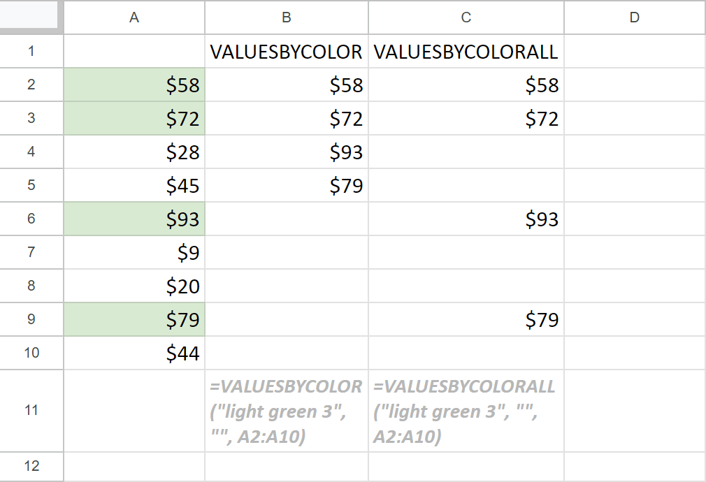
The formulas are in B2 & C2, but you can peek at how they look in B11 & C11:
=VALUESBYCOLOR("light green 3", "", A2:A10)
and
=VALUESBYCOLORALL("light green 3", "", A2:A10)
Tip. The color names are just as they are in the Google Sheets palette:
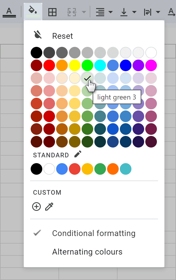
These two functions have the same arguments and even their names are so similar!
Yet, they return different sets of data:
- VALUESBYCOLOR returns the list of only those records that appear with a green fill color in column A. The outcome of this formula takes only 4 cells: B2:B5.
- VALUESBYCOLORALL, in its turn, returns the range of the same size as the original one (9 cells) — C2:C10. However, records in this range appear only for cells with the required fill color in column A. Other cells remain empty.
Even though this may seem the same to you, it makes a huge difference in combination with other functions. And this is exactly what lets you check colors along with the contents of cells with such functions as COUNTIFS or SUMIFS.
Google Sheets CELLCOLOR formulas
This next function is pretty easy. Google Sheets CELLCOLOR formula checks cell colors and returns a list of color names or their RGB codes (it's your choice) for each cell.
You may not need those color names directly but you can use them in other functions, for example, as a condition.
This function also needs 3 arguments:
- range — those cells that you want to check for colors.
- color_source — tells the function where to look at:
- use the word "fill" in double quotes to check for background colors
- "font" — for text colors
- "both" — for both fill and text colors
- color_name — your way of telling what kind of name to return:
- TRUE gets you the names that you see in a Google Sheets palette, e.g. red or dark blue 1
- FALSE gets RGB codes of the colors, e.g. #ff0000 or #3d85c6
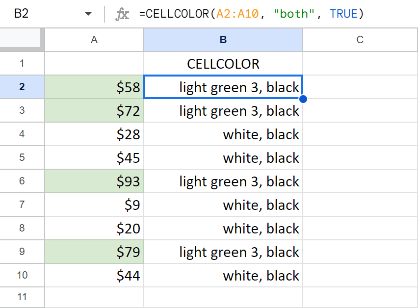
For example, the formula below returns the list of fill and font colors used in each cell of A2:A10:
=CELLCOLOR(A2:A10, "both", TRUE)
So how do you use these functions with IF, SUMIFS, COUNTIFS? How do you set up your search criteria based on colors?
Sum and count cells by color and the contents — formula examples
Let's try and use VALUESBYCOLORALL and CELLCOLOR in a few simple cases.
IF cell color is red, then... — Google Sheets formulas
Here I have a short list of students passing 3 tests:
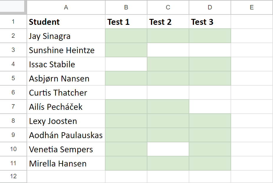
I want to mark the row with PASS in column E only if all cells in a row are green (students who passed all exams). I will use our CELLCOLOR in the IF function to check the colors and return the required string:
=IF(COUNTIF(CELLCOLOR(B2:D2,"fill",TRUE),"light green 3")=3,"PASS","")
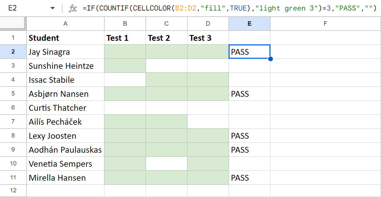
Here's what it does:
- CELLCOLOR(B2:D2,"fill",TRUE) returns all fill colors used in a row.
- COUNTIF(CELLCOLOR(B2:D2,"fill",TRUE),"light green 3")=3 takes those colors and checks if 'light green 3' (in my cells) appears 3 times in a row exactly.
- If so, IF returns 'PASS', otherwise, the cell remains empty.
COUNTIFS: count by colors & values with 1 formula
COUNTIFS is another function that can finally count by multiple criteria even if one of them is color.
Let's suppose there are records of profits per shift and per employee:
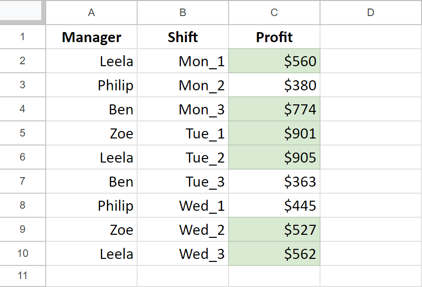
Using our two custom functions inside COUNTIFS, I can count how many times each employee implemented the sales plan (green cells).
Example 1. COUNTIFS + CELLCOLOR
I will list all managers next to the table with data and enter a separate formula for each employee. I'll start with CELLCOLOR:
=COUNTIFS($A$2:$A$10,E2,CELLCOLOR($C$2:$C$10,"fill",TRUE),"light green 3")
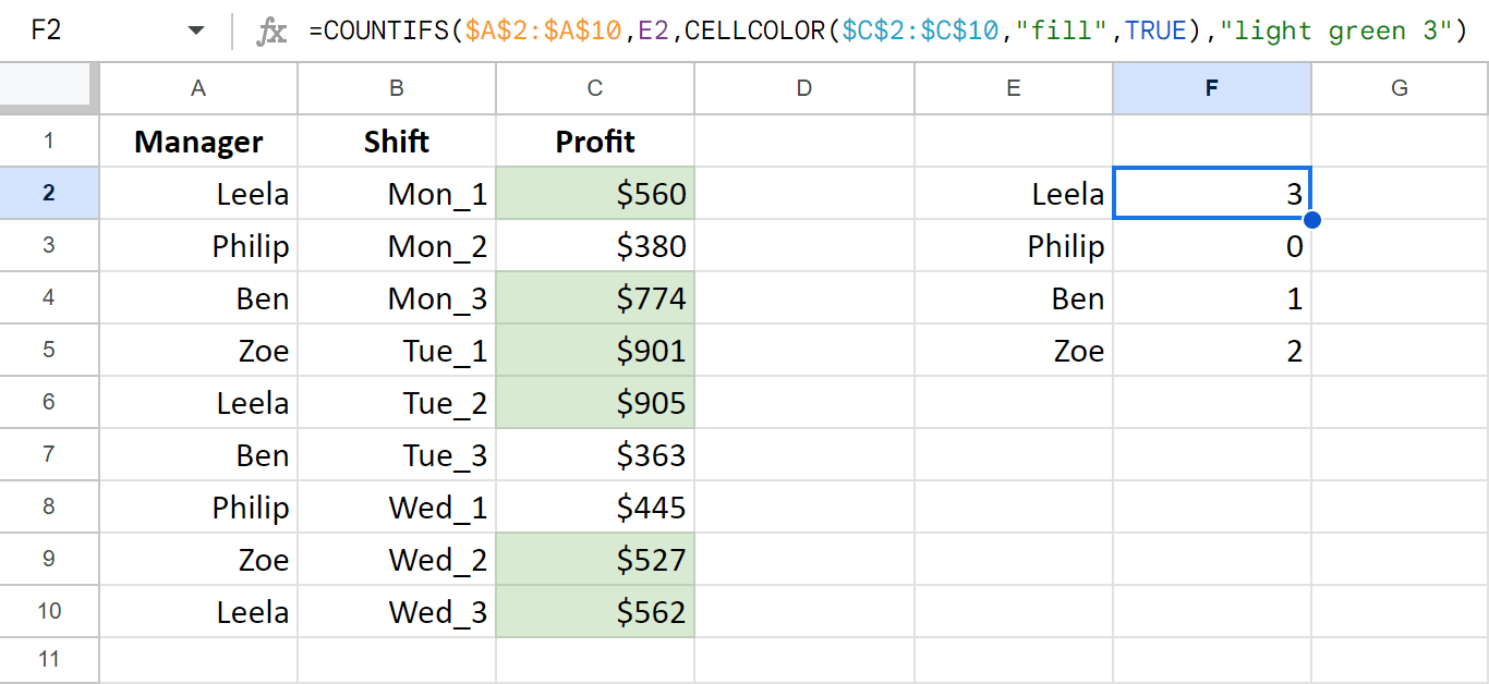
- The first thing the formula checks is cells in column A: if there's 'Leela' (a name from E2), it takes the record into account.
- The second thing it looks for is cells with the 'light green 3' color in column C.
Tip. Check the cell color using the Google Sheets palette:

Since COUNTIFS itself cannot just pick up color, I use our CELLCOLOR as a range for condition.
Remember, CELLCOLOR returns a list of colors used in each cell. When I embed it in COUNTIFS, the latter scans that list searching for all occurrences of 'light green 3'. This in combination with a name from column E gives the required result. Easy peasy :)
Example 2. COUNTIFS + VALUESBYCOLORALL
The same happens if you choose VALUESBYCOLORALL instead. Enter it as a range for the second condition:
=COUNTIFS($A$2:$A$10,E2,VALUESBYCOLORALL("light green 3","",$C$2:C$10),"<>")
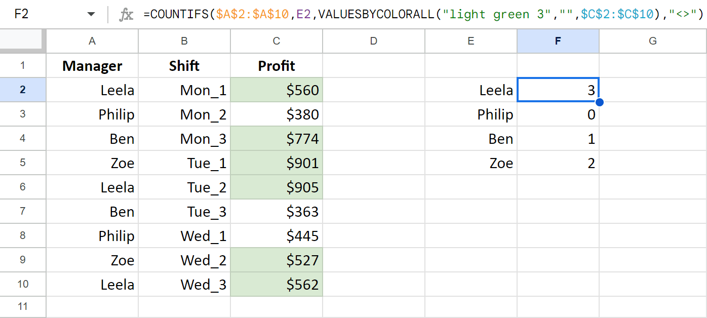
Do you remember what VALUESBYCOLORALL returns? A range of cells where only cells that meet your color requirements contain records. All other cells remain empty.
So when VALUESBYCOLORALL is put to COUNTIFS, the formula counts only those cells that are not empty: "<>" (or, in other words, correspond to the required color).
SUMIFS: sum cells by colors & values with 1 formula
The story with SUMIFS is just like with COUNTIFS:
- Take one of our custom functions: CELLCOLOR or VALUESBYCOLORALL.
- Put it as a range that should be tested for colors.
- Enter the condition depending on the function you selected: the name of the color for CELLCOLOR and "not empty" ("<>") for VALUESBYCOLORALL.
Note. SUMIFS doesn't take anything but a simple range as its first argument — sum_range. If you try and embed one of our custom functions there, the formula just won't work. So keep that in mind and be sure to enter CELLCOLOR and VALUESBYCOLORALL as a criterion instead.
Here are a couple of examples.
Example 1. SUMIFS + CELLCOLOR
Look at this formula:
=SUMIFS($C$2:$C$10,A$2:A$10,E2,CELLCOLOR($C$2:$C$10,"fill",TRUE),"light green 3")
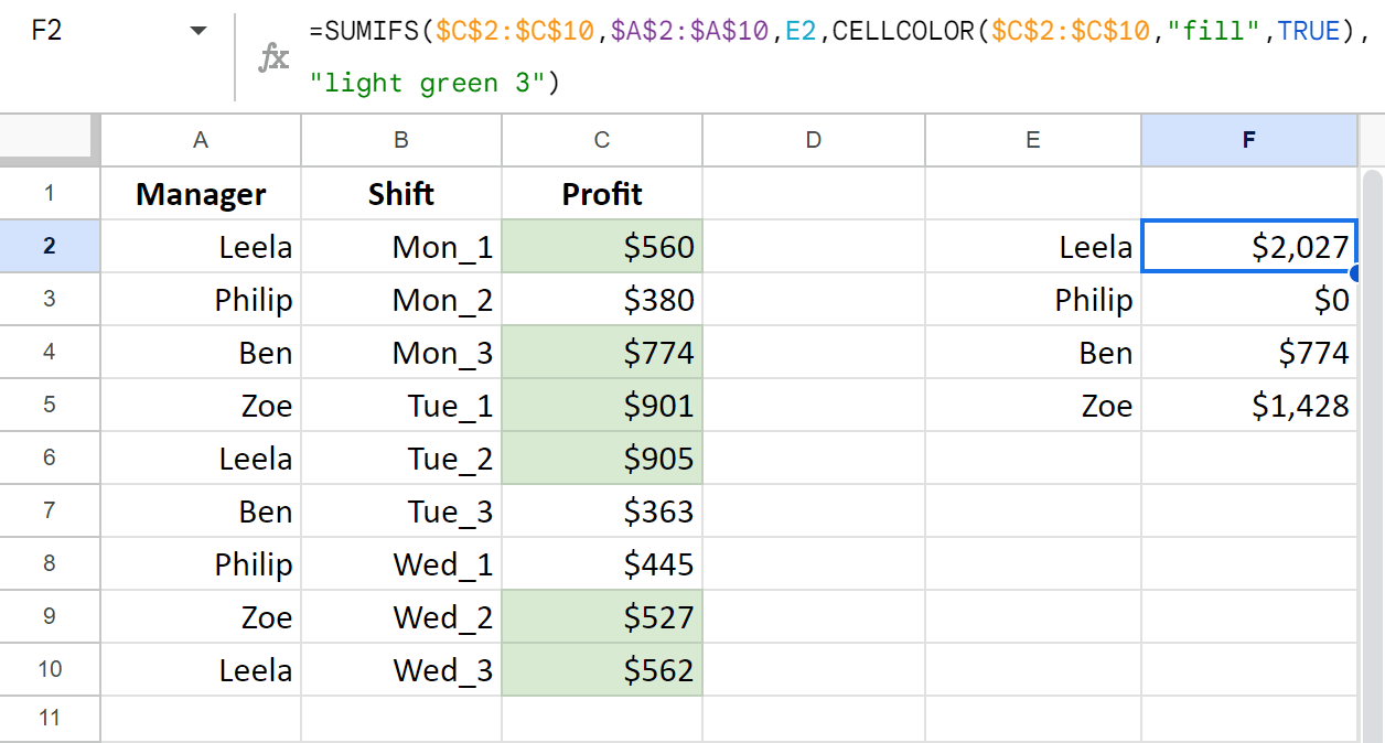
- CELLCOLOR gets all fill colors from C2:C10 and SUMIFS checks if any of them are 'light green 3'.
- SUMIFS also scans A2:A10 for a name from E2 — Leela.
- Once both conditions are met, the total from C2:C10 is ready.
Example 2. SUMIFS + VALUESBYCOLORALL
The same happens with VALUESBYCOLORALL:
=SUMIFS($C$2:$C$10,$A$2:$A$10,E2,VALUESBYCOLORALL("light green 3","",$C$2:$C$10),"<>")
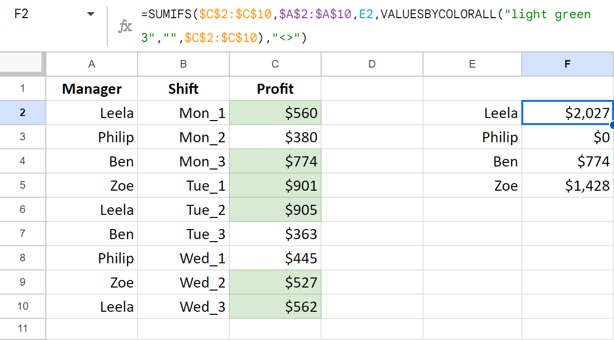
- VALUESBYCOLORALL returns the range where only cells of the required fill color contain values. SUMIFS takes all non-empty cells into consideration.
- SUMIFS also scans A2:A10 for 'Leela' from E2.
- Once both conditions are met, you will get the corresponding total from C2:C10.
Hope this tutorial explains how the functions work and hint at possible ways to use them. If you still have difficulties applying them to your case, meet me in the comments section ;)
Spreadsheet to practice along
Function by Color - custom functions - examples (make a copy of the spreadsheet)
 by
by
13 comments
Hi, excellent extension,
However, as someone already mentioned above, for some reason the third condition in "valuesbycolorall" can't be filled with indirect referencing. I'm trying to reference a filtered range from a different spreadsheet (=Filter(Importrange(_;_);_=_) and this leads to an error message that the range couldn't be found.
Any ideas?
Hi Quala12,
Appreciate your feedback!
We've collected a few more requests and formula examples and are currently investigating the possibility to support such references. But in the meantime, only simple ranges are allowed in the function. I'm really sorry for the inconvenience.
HELLO,
Is it also possible to count cells with different shades of green
HELLO,
Is it also possible to count cells with different shades of green, as i have coloum with no. ranging 10-1 million with conditional formatting colour gradient
Hi!
Each shade is a separate color.
Hi,
Is it not possible to use indirect for referencing the 3d argument, range, in the functions by colour?
I am trying to leverage this for only calculating part of a row. It works when I put the actual date range directly in but not when I create it using cells as reference nor with indirect.
Hi Max,
Could you please give me a couple of examples of the fomrulas that don't work?
Hi Natalia,
I used your COUNTIF and VALUESBYCOLORALL formula, which worked perfectly, then all of a sudden it gave me an error. I did not change the formula by any means, I also did not change anything on the sheet, I was actually busy on another sheet, went back and saw the "all of a sudden error", could you please help with a solution?
These are the ones giving errors:
=COUNTIFS($E$2:$E$21,M2,VALUESBYCOLORALL("#900603","WHITE",$H$2:$H$21),"")
=COUNTIFS($E$2:$E$21,M2,VALUESBYCOLORALL("#900603","WHITE",$I$2:$I$21),"")
=COUNTIFS($E$2:$E$21,M2,VALUESBYCOLORALL("#900603","WHITE",$J$2:$J$21),"")
Of which the correct one looks like this:
=COUNTIFS($E$2:$E$21,M2,VALUESBYCOLORALL("#900603","WHITE",$K$2:$K$21),"")
I have the same error at some other cells, which is exactly the same as shown above and all giving the following error:
"Error
Array arguments to COUNTIFS are of different size."
Thanks in advance
Hi Antoinette,
Sorry, I don't see any difference between formulas that don't work and the one that does. Could you please share your spreadsheet with us directly - support@apps4gs.com? I'll look into the problem.
Hi, Trying to use the countifs and cellcolor functions as stated above.
=COUNTIFS($M$4:$M$60,M3,CELLCOLOR($M$4:$M$60,"fill",TRUE),"magenta")
I absolutely have the data in M4 through M60 counting against the data in M3, with a result of 3 instances.
However I have 7 cells in the range with color magenta but when I change or omit the colors for the M3 matched cells the count does not change. I even tried removing the entire CELLCOLOR statement and it has no impact.
I cannot get the addition of the CELLCOLOR statement to affect the outcome at all.
Hi Blaine,
For me to be able to help you, please share your spreadsheet with the formula that doesn't work correctly with us: support@apps4gs.com.
Note. We keep that Google account for file sharing only and don't monitor its Inbox. Please do not email there. Once you share the file, just confirm by replying to this comment.
I'll look into it.
Hello, could i get some help on counting the amount of rows with data typed in them?
Information may or may not repeat.
I have around 350+ rows of data, of which some are not filled in and merely serve as "separator",plus a row in which the information is not relevant.
Is there a function that can help me count the rows with relevant information (repeated or not)? Is there also a way to make this function automatically update if i add more data on following rows?
Hello Margie,
you can use COUNTIF and count blank/non-blank cells in column A for instance to get the count for rows.
As for making the formula take future rows into account, try using the entire column as a reference (A:A) rather than a particular number of rows (A2:A100).