Today we'll look at how to use VLOOKUP in Excel with many detailed step-by-step examples. You'll learn how to Vlookup from another sheet and different workbook, search with wildcards, and a lot more.
This article begins a series covering VLOOKUP, one of the most useful Excel functions and at the same time one of the most intricate and least understood. We will try to explain the basics in a very plain language to make the learning curve for an inexperienced user as easy as possible. We will also provide formula examples that cover the most typical usages of VLOOKUP in Excel, and try to make them both informative and fun.
Excel VLOOKUP function
What is VLOOKUP? To begin with, it is an Excel function :) What does it do? It searches for the value you specify and returns a matching value from another column. More technically, the VLOOKUP function looks up a value in the first column of a given range and returns a value in the same row from another column.
In its common usage, Excel VLOOKUP searches through your data set based on the unique identifier and brings you a piece of information associated with that unique identifier.
The letter "V" stands for "vertical" and is used to differentiate VLOOKUP from the HLOOKUP function that looks up a value in a row rather than column (H stands for "horizontal").
The function is available in all versions of Excel 365 through Excel 2007.
Tip. In Excel 365 and Excel 2021, you can use the XLOOKUP function, which is a more flexible and powerful successor of VLOOKUP.
VLOOKUP syntax
The syntax for the VLOOKUP function is as follows:
Where:
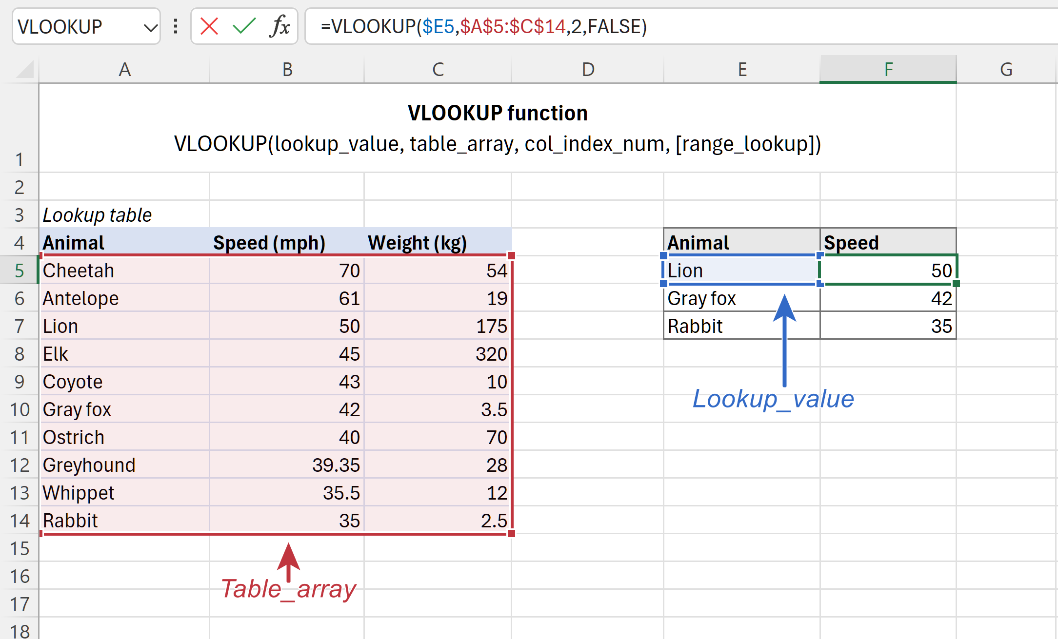
- Lookup_value (required) - is the value to search for.
This can be a value (number, date or text), cell reference (reference to a cell containing a lookup value), or the value returned by some other function. Unlike numbers and cell references, text values should always be in enclosed in "double quotes". - Table_array (required) - is the range of cells where to search for the lookup value and from which to retrieve a match. The VLOOKUP function always searches in the first column of the table array, which may contain various text values, numbers, dates, and logical values.
- Col_index_num (required) - is the number of the column from which to return a value. The counting starts from the leftmost column in the table array, which is 1.
- Range_lookup (optional) - determines whether to search for approximate or exact match:
- TRUE or omitted (default) - approximate match. If an exact match is not found, the formula searches for the largest value that is smaller than the lookup value. Requires sorting the lookup column in ascending order.
- FALSE - exact match. The formula searches for a value exactly equal to the lookup value. If an exact match is not found, a #N/A value is returned.
Basic VLOOKUP formula
Here is an example of the Excel VLOOKUP formula in its simplest form. Please have a look at the below formula and try to "translate" it into English:
=VLOOKUP("lion", A2:B11, 2, FALSE)
- The 1st argument (lookup_value) clearly indicates that the formula looks up the word "lion".
- The 2nd argument (table_array) is A2:B11. Keeping in mind that the search is performed in the left-most column, you can read the above formula a little further: search for "lion" in the range A2:A11. So far, so good, right?
- The 3rd argument col_index_num is 2. Meaning, we want to return a matching value from column B, which is second in the table array.
- The 4th argument range_lookup is FALSE, which indicates that we are looking for exact match.
With all the arguments established, you should have no problem reading the whole formula: search for "lion" in A2:A11, find an exact match, and return a value from column B in the same row.
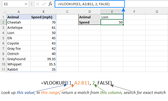
For the sake of convenience, you can type the value of interest in some cell, say E1, replace the "hardcoded" text with the cell reference, and get the formula to look up any value you input in E1:
=VLOOKUP(E1, A2:B11, 2, FALSE)
Does anything remain unclear? Then try looking at it this way:
How to do a Vlookup in Excel
When using VLOOKUP formulas in real-life worksheets, the main rule of thumb is this: lock table array with absolute cell references (like $A$2:$C$11) to prevent it from changing when copying a formula to other cells.
The lookup value in most cases should be a relative reference (like E2) or you can lock only the column coordinate ($E2). When the formula gets copied down the column, the reference will adjust automatically for each row.
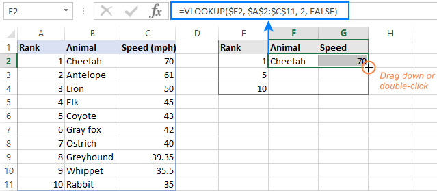
To see how it works in practice, please consider the following example. To our sample table, we have added one more column that ranks the animals by speed (column A) and want to find the 1st, 5th and 10th fastest sprinter in the world. For this, enter the lookup ranks in some cells (E2:E4 in the screenshot below), and use the following formulas:
To pull the animal names from column B:
=VLOOKUP($E2, $A$2:$C$11, 2, FALSE)
To extract speed from column C:
=VLOOKUP($E2, $A$2:$C$11, 3, FALSE)
Enter the above formulas in cells F2 and G2, select those cells, and drag the formulas to the below rows:
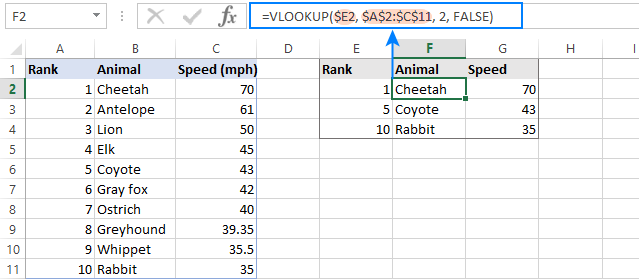
If you investigate the formula in a lower row, you will notice that the lookup value reference has adjusted for that specific row, while the table array is unchanged:
Below, you will have a few more useful tips that will save you a lot of headache and troubleshooting time.
Excel VLOOKUP - 5 things to remember!
- The VLOOKUP function cannot look at its left. It always searches in the leftmost column of the table array and returns a value from a column to the right. If you need to pull values from left, use the INDEX MATCH (or INDEX XMATCH in Excel 365) combination that can does not care about the positioning of the lookup and return columns.
- The VLOOKUP function is case-insensitive, meaning that uppercase and lowercase characters are treated as equivalent. To distinguish the letter case, use case sensitive VLOOKUP formulas.
- Remember about the importance of the last parameter. Use TRUE for approximate match and FALSE for exact match. For full details, please see VLOOKUP TRUE vs. FALSE.
- When searching for approximate match, make sure the data in the lookup column is sorted in ascending order.
- If the lookup value is not found, a #N/A error is returned. For information about other errors, please see Why Excel VLOOKUP is not working.
Excel VLOOKUP examples
I hope vertical lookup is starting to look a bit more familiar to you. To strengthen your knowledge, let's build a few more VLOOKUP formulas.
How to Vlookup from another sheet in Excel
In practice, the Excel VLOOKUP function is rarely used with data in the same worksheet. Most often you will have to pull matching data from a different worksheet.
To Vlookup from a different Excel sheet, put the worksheet's name followed by an exclamation mark in the table_array argument before the range reference. For example, to search in the range A2:B10 on Sheet2, use this formula:
=VLOOKUP("Product1", Sheet2!A2:B10, 2)
Of course, you don't have to type the sheet's name manually. Simply, start typing the formula and when it comes to the table_array argument, switch to the lookup worksheet and select the range using the mouse.
For instance, this is how you can look up the A2 value in the range A2:A9 on the Prices worksheet and return a matching value from column C:
=VLOOKUP(A2, Prices!$A$2:$C$9, 3, FALSE)
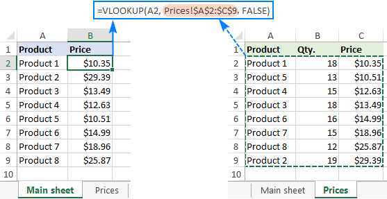
Notes:
- If the spreadsheet name contains spaces or non-alphabetical characters, it must be enclosed in single quotation marks, e.g. 'Price list'!$A$2:$C$9.
- In case you use a VLOOKUP formula for multiple cells, remember to lock table_array with the $ sign, like $A$2:$C$9.
How to Vlookup from another workbook in Excel
To Vlookup from a different Excel workbook, put the workbook's name enclosed in square brackets before the worksheet's name.
For example, here's the formula to look up the A2 value on the sheet named Prices in the Price_List.xlsx workbook:
=VLOOKUP(A2, [Price_List.xlsx]Prices!$A$2:$C$9, 3, FALSE)
If either a workbook name or worksheet name contains spaces or non-alphabetical characters, you should enclose them in single quotes like this:
=VLOOKUP(A2, '[Price List.xlsx]Prices'!$A$2:$C$9, 3, FALSE)
The easiest way to make a VLOOKUP formula that refers to a different workbook is this:
- Open both files.
- Start typing your formula, switch to the other workbook, and select the table array using the mouse.
- Enter the remaining arguments and press the Enter key to complete your formula.
The result will look somewhat like the screenshot below:
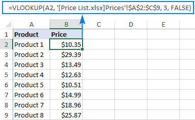
Once you close the file with your lookup table, the VLOOKUP formula will continue working, but it will now display the full path for the closed workbook:
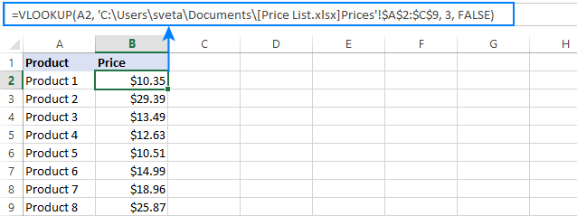
For more information, please see How to refer to another Excel sheet or workbook.
How to Vlookup from a named range in another sheet
In case you plan to use the same lookup range in many formulas, you can create a named range for it and type the name directly in the table_array argument.
To create a named range, simply select the cells and type the name you want in the Name box to the left of the Formula bar. For the detailed steps, please see How to name a range in Excel.
For this example, we gave the name Prices_2020 to the data cells (A2:C9) in the lookup sheet and get this compact formula:
=VLOOKUP(A2, Prices_2020, 3, FALSE)
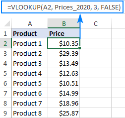
Most names in Excel apply to the entire workbook, so you don't need to specify the worksheet's name when using named ranges.
If the named range is in another workbook, put the workbook's name before the range name, for example:
=VLOOKUP(A2, 'Price List.xlsx'!Prices_2020, 3, FALSE)
Such formulas are far more understandable, aren't they? Besides, using named ranges can be a good alternative to absolute references. Since a named range doesn't change, you can be sure that your table array will remain locked no matter where the formula is moved or copied.
If you have converted your lookup range into a fully-functional Excel table, then you can do a Vlookup based on the table name, e.g. Price_table in the below formula:
=VLOOKUP(A2, Price_table, 3, FALSE)
Table references, also called structured references, are resilient and immune to many data manipulations. For instance, you can remove or add new rows to your lookup table without worrying about updating the references.
Using wildcards in VLOOKUP formula
Like many other formulas, the Excel VLOOKUP function accepts the following wildcard characters:
- Question mark (?) to match any single character.
- Asterisk (*) to match any sequence of characters.
Wildcards prove really useful in many situations:
- When you do not remember the exact text you are looking for.
- When you are looking for a text string that is part of the cell contents.
- When a lookup column contains leading or trailing spaces. In that case, you may rack your brain trying to figure out why a normal formula does not work.
Example 1. Look up text starting or ending with certain characters
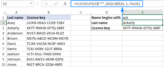
Suppose you want to find a certain customer in the below database. You do not remember the surname, but you are confident that it starts with "ack".
To return the last name from column A, use the following Vlookup wildcard formula:
=VLOOKUP("ack*", $A$2:$B$10, 1, FALSE)
To retrieve the license key from column B, use this one (the difference is only in the column index number):
=VLOOKUP("ack*", $A$2:$B$10, 2, FALSE)
You can also enter the known part of the name in some cell, say E1, and combine the wildcard character with the cell reference:
=VLOOKUP(E1&"*", $A$2:$B$10, 1, FALSE)
The below screenshot shows the results:
Below are a few more VLOOKUP formulas with wildcards.
Find the last name ending with "son":
=VLOOKUP("*son", $A$2:$B$10, 1, FALSE)
Get the name that starts with "joh" and ends with "son":
=VLOOKUP("joh*son", $A$2:$B$10, 1, FALSE)
Pull a 5-character last name:
=VLOOKUP("?????", $A$2:$B$10, 1, FALSE)
Example 2. VLOOKUP wildcard based on cell value
From the previous example, you already know that it is possible to concatenate an ampersand (&) and a cell reference to make a lookup string. To find a value that contains a given character(s) in any position, put an ampersand before and after the cell reference.
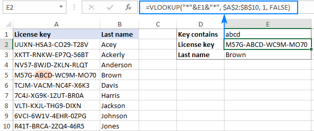
Let's say, you wish to get a name corresponding to a certain license key, but you don't know the whole key, only a few characters. With the keys in column A, names in column B, and part of the target key in E1, you can do a wildcard Vlookup in this way:
Extract the key:
=VLOOKUP("*"&E1&"*", $A$2:$B$10, 1, FALSE)
Extract the name:
=VLOOKUP("*"&E1&"*", $A$2:$B$10, 2, FALSE)
Notes:
- For a wildcard VLOOKUP formula to work correctly, use an exact match (FALSE is the last argument).
- If more than one match is found, the first one is returned.
VLOOKUP TRUE vs FALSE
And now, it's time to take a closer look at the last argument of the Excel VLOOKUP function. Though optional, the range_lookup parameter is highly important. Depending on whether you choose TRUE or FALSE, your formula may yield different results.
Excel VLOOKUP exact match (FALSE)
If range_lookup is set to FALSE, a Vlookup formula searches for a value that is exactly equal to the lookup value. If two or more matches are found, the 1st one is returned. If an exact match is not found, the #N/A error occurs.
Excel VLOOKUP approximate match (TRUE)
If range_lookup is set to TRUE or omitted (default), the formula looks up the closest match. More precisely, it searches for an exact match first, and if an exact match is not found, looks for the next largest value that is less than the lookup value.
An approximate match Vlookup works with the following caveats:
- The lookup column must be sorted in ascending order, from smallest to largest, otherwise a correct value may not be found.
- If the lookup value is smaller than the smallest value in the lookup array, a #N/A error is returned.
The following examples will help you better understand the difference between an exact match and approximate match Vlookup and when each formula is best to be used.
Example 1. How to do an exact match Vlookup
To look up an exact match, just put FALSE in the last argument.
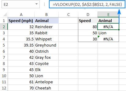
For this example, let's take the animal speed table, swap the columns, and try to find the animals that can run 80, 50 and 30 miles per hour. With the lookup values in D2, D3 and D4, enter the below formula in E2, and then copy it down to two more cells:
=VLOOKUP(D2, $A$2:$B$12, 2, FALSE)
As you can see, the formula returns "Lion" in E3 because they run exactly 50 per hour. For the other two lookup values an exact match is not found, and #N/A errors appear.
Example 2. How to Vlookup for approximate match
To look up an approximate match, there are two essential things you need to do:
- Sort the first column of table_array from smallest to largest.
- Use TRUE for the range_lookup argument or omit it.
Sorting the lookup column is very important because the VLOOKUP function stops searching as soon as it finds a close match smaller than the lookup value. If the data is not sorted properly, you may end up having really strange results or a bunch of #N/A errors.
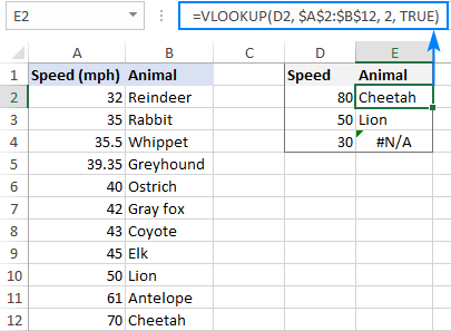
For our sample data, an approximate match Vlookup formula goes as follows:
=VLOOKUP(D2, $A$2:$B$12, 2, TRUE)
And returns the following results:
- For a lookup value of "80", "Cheetah" is returned because its speed (70) is the closest match that is smaller than the lookup value.
- For a lookup value of "50", an exact match is returned (Lion).
- For a lookup value of "30", a #N/A error is returned because the lookup value is less than the smallest value in the lookup column.
Video: How to VLOOKUP in Excel
Step-by-step guidance on how to create and use a VLOOKUP formula in Excel.
Special tools to Vlookup in Excel
Undoubtedly, VLOOKUP is one of the most powerful and useful Excel functions, but it's also one of the most confusing ones. To make the learning curve less steep and experience more enjoyable, we included a couple of time-saving tools in our Ultimate Suite for Excel.
VLOOKUP Wizard - easy way to write complex formulas
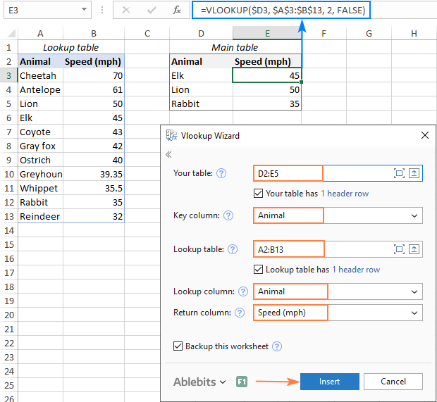
The interactive VLOOKUP Wizard will walk you through the configuration options to build a perfect formula for the criteria you specify. Depending on your data structure, it will use the standard VLOOKUP function or an INDEX MATCH formula that can pull values from left.
To get your custom-tailored formula, this is what you need to do:
- Run the VLOOKUP Wizard.
- Choose your main table and lookup table.
- Specify the following columns (in many cases they are picked automatically):
- Key column - the column in your main table containing the values to look up.
- Lookup column - the column to look up against.
- Return column - the column from which to retrieve values.
- Click the Insert button.
The following examples show the wizard in action.
Standard Vlookup
When the lookup column (Animal) is the leftmost column in the lookup table, a normal VLOOKUP formula for exact match is inserted:
Vlookup to the left
When the lookup column (Animal) is on the right side of the return column (Speed), the wizard inserts an INDEX MATCH formula to Vlookup right to left:
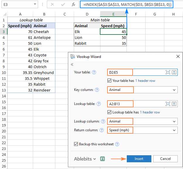
Extra bonus! Due to the clever use of cells references, the formulas can be copied or moved to any column, without you having to update the references.
Merge Two Tables - formula-free alternative to Excel VLOOKUP
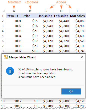
If your Excel files are enormously large and complex, the project's deadline is imminent, and you are looking for someone who can lend you a helping hand, try out the Merge Tables Wizard.
This tool is our visual and stress-free alternative to Excel's VLOOKUP function, which works this way:
- Select your main table.
- Select the lookup table.
- Choose one or several common columns as the unique identifier(s).
- Specify which columns to update.
- Optionally, choose the columns to add.
- Allow the Merge Tables Wizard a few seconds for processing… and enjoy the results :)
That's how to use VLOOKUP in Excel at the basic level. In the next part of our tutorial, we will discuss advanced VLOOKUP examples that will teach you how to Vlookup multiple criteria, return all matches or Nth occurrence, perform double Vlookup, look up across multiple sheets with a single formula, and more. I thank you for reading and hope to see you next week!
Available downloads
Excel VLOOKUP formula examples (.xlsx file)
Ultimate Suite 14-day fully-functional version (.exe file)
 by
by
231 comments
Good morning! I am a Beginner Excel user and need help with Vlookup please in Excel. I have 2 spreadsheets:
Spreadsheet1 has claim numbers in this format:
12345
67890
Spreadsheet2 has the same Claim numbers, but in a new format with a suffix for example:
12345AIAMD00
67890AIAMD01
How do I Vlookup to compare the Base ClaimID from Spreadsheet 2 to Spreadsheet1? Please help, thanks!
Hello!
Use INDEX + MATCH or LOOKUP functions to solve your problem:
=INDEX($F$2:$F$30,MATCH(I2,LEFT($E$2:$E$30,5),0))
=LOOKUP(I2,LEFT($E$2:$E$3,5),$F$2:$F$3)
I2 contains text "12345"
I hope this will help, otherwise please do not hesitate to contact me anytime.
I have a pivot table as follows
A B
1 Labels Count
2 30
3 Malware 2
4 Breach 1
5 Compliance 8
I tried following vlookup formula to get the count of blank label and got an error #N/A instead of actual value 30. Appreciate your help on figuring out the error.
=VLOOKUP("",A:B,2,FALSE)
It works perfectly for labels which are not blank. i.e. =VLOOKUP("Account Issues",A:B,2,FALSE)
Hello!
The VLOOKUP function looks for a specific value. It cannot search for an empty value. You can use the SUMIF function to count by null values.
Alternating between reading the information and doing it in Excel at the same time for almost an hour, I finally got the result that I wanted! Thank you for teaching us noobs :)
I am trying to lookup a value in a column that contains the results of a MID function and I get #N/A. If I use Ctrl F(Find), It will not find the value but if I change the Option from formula to value, it will find the value I am looking for. How can I find my value using vlookup?
Hello Eloisa!
I’m sorry but your task is not entirely clear to me. For me to be able to help you better, please describe your task in more detail. Please specify what you were trying to find, what formula you used and what problem or error occurred. Give an example of the source data and the expected result.
It’ll help me understand it better and find a solution for you. Thank you.
I want to fetch return from row in stead of column. please help me in this regards by providing the example
=vlookup(E1,A2:B6,2,FALSE)
here 2 : return a match from this column
but i want to pick a match from row in that case what will be the formula
Thanks in advance
Hello!
I’m sorry but your task is not entirely clear to me.
For me to be able to help you better, please describe your task in more detail. Please let me know in more detail what you were trying to find. Explain "i want to pick a match from row". Give an example of the source data and the expected result. It’ll help me understand it better and find a solution for you. Thank you.
I'm looking for a formula to return the following, in column b I have a list of tasks,in another column say j these have a a number 1 for complete 0 or incomplete, how to I cross reference the column and description to fill a column on another sheet, I can't get it to return more than one result?? Thanks
If I understand your task correctly, pay attention to the following paragraph of the article in our blog:
https://www.ablebits.com/office-addins-blog/vlookup-multiple-values-excel/#vlookup-multiple-values-columns
I hope this will help, otherwise please do not hesitate to contact me anytime.
Excellent tutorial on Vlookup. Lucidly explained and precise. Topics covered pretty much every thing and impressive.
This formula is extremely awful! I keep getting few arguments, I'm doing evaluation by my school teachers and this keeps happening to me! I tried your formula and nothing worked at all!
I am impressed with vlookup method but i have a problem of how to apply it! I have two sheets of workers, my intension was to send data of workers (454)to my boss but what has been sent are only 435 workers, my question is how can I use vlookup to identify the names which were not sent?
i learn everday and i learn many things
DEAR SIR
I AM RAVI , NOW I AM WORKING VLOOKUP FORMULA ,I WANT TO FIX THE LOOK UP VALUE , HOW ITS WORK
Is there a way of looking up a rate of pay (for an individual worker) from a table where there are multiple agencies, multiple classes of worker (e.g. Healthcare assistant, nurse, doctor) and the rate varies depending on the time/day? Thanks!
My formula is not working. I am using Vlookup to search in a differente workbook and Iall I am getting is "#REF". Already check the column's format and validated instruction. I am not sure what is wrong.
=VLOOKUP(C3,'[Plan Membership Comparison.xls]Sheet5'!$A$2,5)
Hi Roxanna,
In the table_array argument, you need to supply a lookup range, while you only have a single cell ($A$2).
How can I find a texts with same first 2 characters and return the value?
like
ASD-12345
ASD-o9093
DFD-00000
Am I able to search to return the results only with ASD-xxxx? Thank you
How can select the data at a time vlookup results
Madam,
How can i attach data from datasheet of other folders?
MADAM HOW CAN I USE VLOOKUP FORMULA IN MULTI SHEETS?
Hi I am using this formula to look up herbicide name by active ingredient
=LOOKUP(CO80,'Herb list2'!$A$2:$B$77,'Herb list2'!$B$2:$B$77)
IS there any way to change this formula to set to exact match (FALSE)??
I tried
=LOOKUP(CO80,'Herb list2'!$A$2:$B$77,'Herb list2'!$B$2:$B$77, FALSE) an got error msg
"You've entered too many arguments for this function"
U R right lots of headaches!!
Hello
please make a video for this
Hi Samsoor,
We already a video for this, and you can find it here:
https://www.youtube.com/watch?v=Oo-TELIU8XQ&t=1s
I found this site very useful, wherever i forgot or stuck somewhere, it help me solve my problems. Thanks and best regards,
I am happy with your excel examples thank you and need more examples for learning
need further clarification please
I am not able to filter my spreadsheet, i have value 1 to 1000 numbers but i want to filter it based on some random numbers or list of random number.
How i can do it excel. Please suggest for the same.
Appreciate your help.
My VLookup isn't working. I run a report in a software that copies data into an Excel file. I then save the file as an Excel Workbook, and re-open the file in the same instance as my other workbook.
I then copy the data to my other excel workbook, where I have a VLOOKUP set up that references the descriptions of the data with their category code (which isn't included on the original report). However, I'm getting the #N/A error type.
I double checked the formatting and it's identical. Spelling and spacing is also identical. What's odd is, if I delete the data and re-type it into the space the VLookup works. I'd prefer not having to do that each time and am wondering what else might be causing this?
My question above is urgent. Thank you.
Hello,
I got zero results in my VLOOKUP formula. My formula is =IF([Insurance Charge]="Yes",120, IF(E2="No",0,VLOOKUP(E2,G2,'Rental Information'!A3:D7,FALSE))) And the question is Use an exact-match VLOOKUP function nested in an IF function to return the monthly insurance charge if the renter has purchased insurance (“Yes” in the Insurance column). Use the furniture’s Group Code in the Rental Data worksheet and the Monthly Insurance column in the Rental Information worksheet Furniture Rental Charges table (predefined name RentalCharges) to return the appropriate charge. If the renter has not purchased insurance, return 0. Don’t forget to multiply it by the Rental Period to get the final amount.
What's wrong with my formula?
i have 2 coloms in one colom have absenties names and another column have full name list, how i can find presents name list from both list
Thawfeeque:
Depending on what you want to accomplish there are a couple of things you can do with find duplicates.
Go to this address and see if it helps. If you still have questions post them and someone will try to help.
https://www.ablebits.com/office-addins-blog/excel-compare-two-columns-matches-differences/#highlight-matches-differences
How i can get the corrosponding value of column B , column C and column D in sheet 1 from sheet 2 with excel formula. Value In column A of both the sheet are matching but not serial wise.
Thank you for such a clear and easy to understand training. Most appreciated.
need to know how to copy and paste some cells from a page of a spread sheet to an email WITHOUT any formula data included and look exactly as the copied cells
Select your entire spreadsheet, do a copy paste, next do a copy paste special and choose Values. Once you do this the exact number and not the formula will paste to your spreadsheet.
Thank you! This is VERY helpful!
VLookup expanded here is "Too" Complicated..!!!
'v-03'!H33 I have four formulas that are similar but only one doesn't calculate total please help
Explain V lookup together to Choose function Any Example?
Hi Maina,
We published a separate tutorial on Excel CHOOSE function with formula examples. Hope you will find it useful :)
Helpful excel,but can you sheet provide for website.
Thanks
How would I use vlookup formula to access various files - ie I want the user to enter in the file name into a cell (A1) and the various VLOOKUP formulas would use the A1 text to feed into the external file reference.
example:
=VLOOKUP("Die Size", 'C:\Users\Dwayne\Desktop\[(A1).xlsx] Set-up'!$A$16:$AB$16,13,TRUE)
And in this case the A1 is a cell reference in the same worksheet; and then the user could get the various info without editing every formula.
advice appreciated!
If the unique identifiers is repeated a few time in the table for example "Product1" appears three times and I would like the corresponding data or all three times it appears, may I know how it can be done. The three corresponding data is text and should appear on three different lines. Thanks for your help.
Hi Adrian,
The VLOOKUP function cannot return multiple matches, you'd need an array formula for that. A few formula examples can be found here: How to Vlookup multiple matches in Excel.
hello
please help me.
Big thanks to Microsoft for inventing vlookup function.
As a Senior manager I rely on this, not my staff.
They all leave me. They hate me.
I have to register daily sales details, for example 01-01-2018 Raju sales in rupees Rs.1000/-, Ramu sales in rupees Rs.1500/-, now I need 01-01-2018 individual sales amount in another sheet
You may do with helper column which you will put serial number to make each 01-01-2018 unique then the lookup formular will use those unique ref to pull their respective sales
Hello! I have a VLookup that I am using with the IF function to pull pay rates (regular/overtime) and match it with employee names. My data is in 3 columns (Employee,Reg. Rate, OT Rate) and the lookup is checking 2 columns (Employee, Pay Type) for data. It's working great EXCEPT, I cannot get the N/A to hide if the columns are blank. Below is the current formula:
=IF(B8="overtime", VLOOKUP(A8, EmployeeRates, 3, FALSE), VLOOKUP(A8, EmployeeRates, 2, FALSE))
Any help would be greatly appreciated.
=iferror(IF(B8="overtime", VLOOKUP(A8, EmployeeRates, 3, FALSE), VLOOKUP(A8, EmployeeRates, 2, FALSE)),o)
Your wildcard examples work on no data, but the exact values you used in your example. I tried to replicate your using the cell contents example with the animal table using =VLOOKUP("*"&C1&"*",$A$2:$B$13, 1,FALSE) where C1 has Coy typed into it. It should find "Coyote" and return the speed but it does not. I cannot figure out what is going wrong.
Hello TC,
We have uploaded the VLOOKUP sample worksheet with all the formula examples, so you can check the wildcard formulas.
How do I identify records from one worksheet A which is not in worksheet B and then copy only those record from A to B which is not in B.Please help.
Thanks
So I need to run a report where I need to count up how many times an item shows up across 12 different sheets (each sheet is a month of data). Is there a way to use vlookup to look in an entire workbook without having to input every worksheet name in the formula?
Hello, Jason,
If you need to count up how many times an item shows up in your sheets, please try the combination of COUNTIF and SUMPRODUCT functions. First you need to create a range containing the names of the relevant sheets, and then use the following formula:
=SUMPRODUCT(COUNTIF(INDIRECT("'"&A2:A14&"'!A2:A10"),C2))
Where &A2:A14& is the list with the sheets names; A2:A10 is the data range that you want to count the specified value across worksheets; C2 is the cell with the value you want to count up.
Hope this will help.
I am trying to reference another spreadsheet with the name of customers in Column B and needing to reference their spending which is located in column D and divide column D by 4. There are 700+ customers so I want to ensure that I reference the correct customer with their spending instead of having to key all manually.
Any help you can provide will be greatly appreciated.
Hello, Deb,
I'm sorry, it is not very clear what result you want to get. Could you please describe your task in more detail and send us a small sample workbook with the source data and expected result to support@ablebits.com? I kindly ask you to shorten your tables to 10-20 rows/columns and include the link to your blog comment.
We'll look into your task and try to help.
I am trying to reference another spreadsheet with the name of customers in Column B and needing to reference their spending which is located in column D and divide column D by 4.
Any help you can provide will be greatly appreciated.
I can't get my Vlookup to work. I used the same formula last year with no issues. I have excel 2016. I have 2 sheets in one workbook and here is my formula
=VLOOKUP(A2,'Pay Register Total'!A$2:F$1762,6,FALSE)
The formula returns #N/A on every line.
I have the same data, supplier number, in the first column on both sheets.
Please help!!
thanks,
Margaret
Check the format of each column being used in your Vlookup. The #N/A often results due to formatting mismatch.
I think you are point 7 inverted.
7. And finally, remember about the importance of the last parameter. Supply TRUE for exact match or FALSE for approximate match, and it will save you a lot of headache.
Hi Suhendra,
Good catch, thank you! Fixed.
I knew there had to be a way to look up one cell and then return a neighboring cell, and I found it here. Thank you so much for this simple tutorial, it saved me a ton of time!
I've solved it, realised should be TRUE instead of FALSE thanks anyway