Recently we have published a few articles covering different aspects of Excel conditional formatting. Unexpectedly, it's turned out that it's not creating a rule and even not making a proper formula that represents the greatest challenge. Using proper cell references in Excel formulas appear to be the most complex part and a common source of problems.
"I had my conditional rule correct, except for the mixed references." This is what our blog readers have often reported in comments. So, why don't we invest a few minutes to figure this thing out? This will certainly save you far more time in the long run!
How relative and absolute cell references work in conditional formatting rules
In all Excel formulas, including conditional formatting rules, cell references can be of the following types:
- Absolute cell references (with the $ sign, e.g. $A$1) always remain constant, no matter where they are copied.
- Relative cells references (without the $ sign, e.g. A1) change based on the relative position of rows and columns, when copied across multiple cells.
- Mixed cells references (absolute column and relative row (e.g. $A1), or relative column and absolute row (e.g. A$1). In Excel conditional formatting rules, mixed cell references are used most often, indicating that a column letter or row number is to remain fixed when the rule is applied to all other cells in the selected range.
In Excel conditional formatting, cell references are relative to the top-left cell in the applied range . So, when making a new rule, you can simply pretend as if you are writing a formula for the upper-left cell only, and Excel will "copy" your formula to all other cells in the selected range. If your formula refers to a wrong cell, a mismatch between the active cell and the formula will occur, which will result in conditional formatting highlighting wrong cells.
Now, let me show you a few examples that demonstrate how seemingly identical formulas produce different results depending on what cell references types are used.
Example 1. Absolute column and relative row
This pattern is most typical for conditional formatting rules and in 90% of cases cell references in your Excel conditional formatting rules will be of this type.
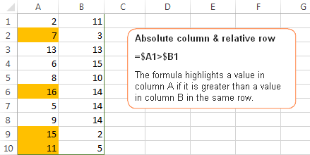
Let's make a very simple rule that compares values in columns A and B and highlights a value in column A if it is greater than a value in column B in the same row.
If you need the detailed instructions on how to create conditional formatting rules with formulas, here you go - Creating an Excel conditional formatting rule using a formula. In this case, the formula is obvious:
=$A1>$B1
Because you always compare values in columns A and B, you "fix" these column by using absolute column references, notice the $ sign before the column letters in the above formula. And, since you are comparing the values in each row individually, you use relative row references, without $.

Example 2. Relative column and absolute row
This cell reference type is the opposite of the previous one. In this case, the row number is always constant while the column changes. You use such references when you want to check values in a given row against a certain value or against values in another row.
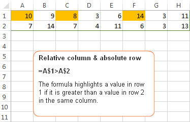
For example, the below formula compares values in row 1 and 2 and the rule highlights a value in row 1 if it is greater than a value in row 2 in the same column:
=A$1>A$2

Because you want the row numbers to be fixed, you use the absolute row references, with the $ sign. And, because you want to compare values in each column individually, you create the rule for the left-most column (A) and use relative column references, without the $ sign.
Example 3. Absolute column and absolute row
You use absolute row and absolute column references if you want to compare all values in the selected range with some other value.
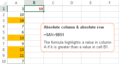
For example, let's create a rule that highlights all values in column A that are greater than a value in cell B1. The formula is as follows:
=$A1>$B$1
Please pay attention to the use of the following references:
- $A1 - you use an absolute column and relative row references because we want to check values in all cells of column A against the value in cell B1.
- $B$1 - you use absolute column & absolute row because cell B1 contains the value you want to compare all other values against and you want this cell reference to be constant.

Example 4. Relative column and relative row
This reference type is used in Excel conditional formatting rules least of all. You use relative column & relative row references when you want to check all cells of the selected range against a certain value.
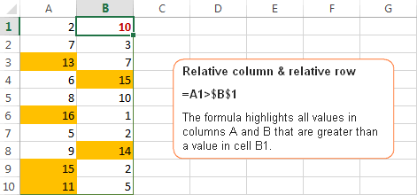
Suppose, you want to highlight all cells in columns A and B that are greater than a value in cell B1. You can simply copy the formula from the previous example and replace $A1 with A1 since you do not want to fix either row or column:
=$A1>$B$1
Remember, you write the formula for the top-left cell in your range, A1 in our case. When you create a rule with the above formula and apply it to some range, say A1:B10, the result will look similar to this:

Tip. To quickly toggle between absolute and relative references, select the cell reference in the formula bar and press the F4 function key. The reference will rotate between the four types from relative to absolute, like this: A1 > $A$1 > A$1 > $A1, and then back to the relative reference A1.
Hopefully, these simples examples have helped you fathom out the essence of relative and absolute cell references in Excel. Now that you know how to determine the appropriate reference type for your rules, go ahead and harvest the power of Excel conditional formatting for your projects. The following resources may prove helpful.
 by
by
96 comments
^^^Sorry I just posted below, but after checking General vs Number formatting, I entered this new to add another condition and it started to work. I have no clue why.
=OR(O2="FLEXPT",O2="FLEXRT")
Whit this formula ONLY those cells are highlighted.
This simple conditional format formula, =(O2="FLEXPT"), is not only highlighting cells that contain FLEXPT, but also highlighting cells that contain NF6-0120, NN2-0120, RT6061-1, etc. This is the only Conditional Formatting rule in the workbook (single sheet). Can you explain why? Thank you.
Hi! I can't see your data. So I can't tell you the exact cause of the error. However, you should check your conditional formatting formula and the range that you are formatting. The formula should have a reference to the first cell in the conditional formatting range. Read more: Excel Conditional Formatting tutorial with examples.
Hi, I am trying to apply conditional formatting to a table. each column has a range at the top of the column in a separate table
for context as I think itll help, I am tracking medical blood test results like hemoglobin etc. so for ex A2 will be max range and A3 will be min range and then A7 downwards will be the results on different days.
So I am able to set up conditional formatting for each column by choosing conditional formatting, highlight cell rules, more rules, format only cells that contain cell value not between A2 and A3. the problem is it automatically makes this absolute cell reference and doesn't allow me to change it so i cannot use format painter.
I have too many columns to do this for each one (over 50 - imagine all blood results!)
Is there another way to go about this?
Hi! Try applying the column A conditional formatting formula to the entire range at once (e.g. A1:AZ50). You can also try copying the conditional formatting. Read more: How to copy Excel conditional formatting.
I'm having trouble where I have a column C with the total difference of Column B - Column A and then for the totals in column C I need a conditional formatting to put in colors for that cell depending on the total. It is not letting me do the conditional formatting and the formula at once, is there a way to do that?
Hello! Conditional formatting cannot prevent the execution of formulas in cells. You can calculate formulas and perform conditional formatting at the same time. Maybe this article will be helpful: Excel Conditional Formatting tutorial with examples.
Your example 4 is wrong. You call it relative column and rows, but in your example you have references to absolute formulas.
Note that the example shows changing the relative reference in A1. The difference between relative and absolute references is shown by using an absolute reference in B1.
I've formatted cell E7 to change colors relative to C7, for example if E7>C7*.1, cell turns green or whatever. Got that all to work great. I want to copy it to cell E8 relative to C8, but it seems like anything I do keeps making it relative to C7. How can I make E8 be relative to C8, E9 to C9, etc. without having to just manually re-enter the formula in each cell
Hi! I recommend reading this guide: Excel conditional formatting formulas based on another cell. Select the range of cells for conditional formatting in column E. Use this conditional formatting formula:
=E1>C1*0.1
You can also find useful information in this guide: Copy conditional formatting.
Super helpful - >8 MS support explanations and still did not make it clear - you nailed it right out of the gate.
Hey, so my problem is like this:
MONDAY TUESDAY WEDNESDAY THURSDAY FRIDAY Total
SP
SFFNR
SFAM
SFNRL
SICK
Total
Now, I want to take the number of SPs in Mondays, number of SFFNR's in Monday and so on, same with the number of Tuesdays in SPs. I am using COUNTIFS function for this and I want to change the only the row numbers(SP, SFFNR, SFAM....) when i'm copying the formula downside but at the same time i want to change only the column numbers when i copy it horizontally or right side like(Monday, tuesday, wednesday...)
Hi!
Here is the article that may be helpful to you: How to copy formula in Excel with or without changing references.
Thank you, that was a lifesaver.
created a Conditional Formatting Rule that will highlight the cell if any of the values in the range A3:A50 meets or exceeds the new Client Goal of 3 in cell A1, using this Rule: “=$A$3>=$A$1”. However, the formatting was changed for the entire range whether the criteria was met or not.
Hi!
If I understand the issue correctly, this conditional formatting formula will highlight every cell that is greater than or equal to A1. You can apply this conditional formatting to the range A3:A50.
=A3>= $A$1
If this is not what you wanted, please describe the problem in more detail.
Hey
I have the follow sheet 1, with ID and city/country names:
1234 Sydney
5678 Kimberly
9191 Milan
1213 Denmark
1415 England
1617 France
1819 Sudan
2021 Greece
2023 Ghana
2425 China
And i have the following sheet 2:
1234
2425
5678
2023
9191
2021
1213
1819
1415
1617
2777
2344
I would like to copy the city/country names from sheet 1, according to their associated ID sheet 1 - wich would make sheet 2 look as following:
1234 Sydney
2425 China
5678 Kimberly
2023 Ghana
9191 Milan
2021 Greece
1213 Denmark
1819 Sudan
1415 England
1617 France
2777
2344
Hello!
The formula below will do the trick for you:
=IFERROR(VLOOKUP(A1,Sheet1!$A$1:$B$10,2,0),"")
You can learn more about VLOOKUP function in Excel in this article on our blog.
Thank you so much for this page!!! I have searched multiple times and spent hours trying to figure out how to do this - apply a conditional formatting rule comparing values of two columns on each row. Yours is the only explanation I found that was so written so clearly and with such good examples, that I was able to make the change I needed within a few seconds of finishing reading! I changed my rule from Cell Value = $A$2 to Cell Value = $A2 and left the Applies to =$C$2:$C$411 and every matching columns had the formatting (color green) on each row and every non-matching columns on the row were not colored green. I can't thank you enough!!!
I have two lists of numbers in adjacent rows, and want to apply conditional formatting to the bottom row such that it colours the cell green if that number is within a bound of 100 either side of the relevant number in the top column, yellow if a further 100 above or below the previous bound, and red if any further out than that.
I want this conditional formatting to hold for all cells within these two rows, and format each cell in the bottom row depending solely on the cell directly above it.
I'm afraid I'm at a bit of a loss at this point, and without any support, I will have to input this manually for every cell in the range - any help would be much appreciated.
Hello!
If I understand your task correctly, the following formula conditional formatting should work for you:
=ABS(A1-A2) =< 100
the formula for the second condition is
=ABS(A1-A2) =< 200
the formula for the third condition is
=ABS(A1-A2) > 200
Create conditional formatting with these rules for cell A2. Then copy the format to other cells.
Thank you for all your wonderful blogs! They have helped me a lot! Thanks!
Hai,
Please give me your suggestion in excel on below mentioned condition
Source cell value is 35 (A1)
I will enter 0 to 25 (number) in cell A2 then this cell color will change red automatically and entered 26 to 35 then change green color automatically based on A1 cell value. It is possible.
Hello Ramkrish!
I recommend studying this article on conditional formatting on our blog.
I have searched extensively and cannot find the answer to my HOW-To COnditional Formatting question/need.
I have two sheets in the spreADSHEET, each contains the identical BUDGET spreadsheet. (12 MOnths across top and 30 budget categories along the left side.)
They are identical now when I create the budget, but one will be used to record aCTUAL expenses as the year progresses. I want to use COnditional Formatting on each cell, to highlight when that cells amount exceeds (>) then Budget Sheet's value for that same cell.
I use formula =D15>(BUDGET!$D15*1.05) and then highlight red.
When I use Format Painter across a row or column, EXCEL fixes that original D15 reference.
I want the test cell reference to change relatively too.
Does anyone follow this and have a solution for me?
How do you round the sum of a column of numbers in the same box that you used the relative formula for? I keep getting errors.
Hi! Attempting to apply a 3-color scale to a column of values where the formatting only applies to the previous n cells. New data is added to the column daily and I want the formatting to follow where it only works on the previous n cells. I think of it like a "running average" format. The problem seems to lie with the fact that Excel will only allow absolute references when determining to which cells the rule applies. If they were relative references, it would be perfect.
It was really helpful.
Thank you Svetlan Cheusheva
Hello Svetlana,
WOULD YOU TELL ME ABOUT THE SOLUTION OF FOLLOWING PROBLEM:
COLUMN NO D G W X
ROW NO. 33 33 33 33
REF. CELL NO. D33 G33 W33 X33
HOW I'LL USE THESE CELL NO. ie. D33, G33, W33, X33 IN THE FORMULA WHICH VALUE WILL BE DIFFERENT ON BASIS OF ROW NO. 33 (IT MAY BE OTHER LIKE 42, 12 ETC)
THANKS FOR YOUR PATIENCE.