This tutorial shows how to use INDEX and MATCH in Excel and how it is better than VLOOKUP.
In a couple of recent articles, we made a good effort to explain the basics of VLOOKUP function to beginners and provide more complex VLOOKUP formula examples to power users. And now, I will try if not to talk you out of using VLOOKUP, then at least show you an alternative way to do a vertical lookup in Excel.
"What do I need that for?" you may wonder. Because VLOOKUP has numerous limitations that can prevent you from getting the desired result in many situations. On the other hand, the INDEX MATCH combination is more flexible and has many awesome features that make it superior to VLOOKUP in many respects.

Excel INDEX and MATCH functions - the basics
Since the aim of this tutorial is to demonstrate an alternative way to do a vlookup in Excel by using a combination of INDEX and MATCH functions, we won't dwell much on their syntax and uses. We will cover only the minimum necessary for understanding the general idea and then take an in-depth look at formula examples that reveal all the advantages of using INDEX MATCH instead of VLOOKUP.
INDEX function - syntax and usage
The Excel INDEX function returns a value in an array based on the row and column numbers you specify. The syntax of the INDEX function is straightforward:
Here is a very simple explanation of each parameter:
- array - a range of cells that you want to return a value from.
- row_num - the row number in array from which you want to return a value. If omitted, the column_num is required.
- column_num - the column number in array from which you want to return a value. If omitted, row_num is required.
For more information, please see Excel INDEX function.
And here is an example of the INDEX formula in its simplest form:
=INDEX(A1:C10,2,3)
The formula searches in cells A1 through C10 and returns a value of the cell in the 2nd row and the 3rd column, i.e. cell C2.
Very easy, right? However, when working with real data you would hardly ever know which row and column you want, that's where the MATCH function comes in handy.
MATCH function - syntax and usage
The Excel MATCH function searches for a lookup value in a range of cells and returns the relative position of that value in the range.
The syntax of the MATCH function is as follows:
- lookup_value - the number or text value you are looking for.
- lookup_array - a range of cells being searched.
- match_type - specifies whether to return an exact match or the nearest match:
- 1 or omitted (default) - approximate match (next smaller).
- 0 - exact match. In the INDEX / MATCH combination, you almost always need an exact match, so you set the third argument of your MATCH function to 0.
- -1 - approximate match (next larger).
For example, if the range B1:B3 contains the values "New-York", "Paris", "London", the below formula returns the number 3, because "London" is the third entry in the range:
=MATCH("London",B1:B3,0)
For more information, please see Excel MATCH function.
At first sight, the usefulness of the MATCH function may seem questionable. Who cares about the position of a value in a range? What we do want to know is the value itself.
Let me remind you that the relative position of the lookup value (i.e. row and column numbers) is exactly what you need to supply to the row_num and column_num arguments of the INDEX function. As you remember, Excel INDEX can find the value at the juncture of a given row and column, but it cannot determine which exactly row and column you want.
How to use INDEX MATCH function in Excel
Now that you know the basics, I believe it has already started making sense how MATCH and INDEX work together. In a nutshell, INDEX finds the lookup value by column and row numbers, and MATCH provides those numbers. That's it!
For vertical lookup, you use the MATCH function only to determine the row number and supply the column range directly to INDEX:
Still having difficulties to figure that out? It might be easier to understand from an example. Suppose you have a list of national capitals and their population:
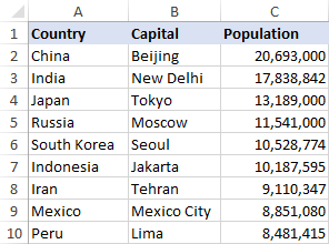
To find the population of a certain capital, say the capital of Japan, use the following INDEX MATCH formula:
=INDEX(C2:C10, MATCH("Japan", A2:A10, 0))
Now, let's analyze what each component of this formula actually does:
- The MATCH function searches for the lookup value "Japan" in the range A2:A10, and returns the number 3, because "Japan" is third in the lookup array.
- The row number goes directly to the row_num argument of INDEX instructing it to return a value from that row.
So, the above formula turns into a simple INDEX(C2:C,3) that says to search in cells C2 through C10 and pull the value from the 3rd cell in that range, i.e. C4 because we start counting from the second row.
Don't want to hardcode the city in the formula? Input it in some cell, say F1, supply the cell reference to MATCH, and you will get a dynamic lookup formula:
=INDEX(C2:C10, MATCH(F1,A2:A10,0))
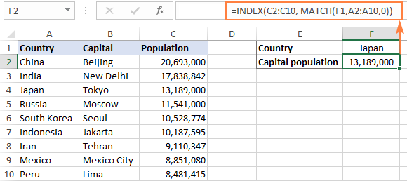
Important note! The number of rows in the array argument of INDEX should match the number of rows in the lookup_array argument of MATCH, otherwise the formula will produce an incorrect result.
Wait, wait… why don't we simply use the following Vlookup formula? What's the point in wasting time trying to figure out the arcane twists of Excel MATCH INDEX?
=VLOOKUP(F1, A2:C10, 3, FALSE)
In this case, no point at all :) This simple example is for demonstration purposes only, so that you get a feel of how the INDEX and MATCH functions work together. Other examples that follow below will show you the real power of this combination that easily copes with many complex scenarios when VLOOKUP stumbles.
Tips:
- In Excel 365 and Excel 2021, you can use a more modern INDEX XMATCH formula.
- For Google Sheets, see formula examples with INDEX MATCH in this article.
INDEX MATCH vs. VLOOKUP
When deciding which function to use for vertical lookups, most Excel gurus agree that INDEX MATCH is far better than VLOOKUP. However, many people still stay with VLOOKUP, firstly, because it's simpler and, secondly, because they do not fully understand all benefits of using the INDEX MATCH formula in Excel. Without such understanding no one is willing to invest their time to learn a more complex syntax.
Below, I will point out the key advantages of MATCH INDEX over VLOOKUP, and you decide whether it's a worthy addition to your Excel arsenal.
4 main reasons to use INDEX MATCH instead of VLOOKUP
- Right to left lookup. As any educated user knows, VLOOKUP cannot look to its left, meaning your lookup value should always reside in the leftmost column of the table. INDEX MATCH can do left lookup with ease! The following example shows it in action: How to Vlookup a value to the left in Excel.
- Insert or delete columns safely. VLOOKUP formulas get broken or delivers incorrect results when a new column is deleted from or added to a lookup table because VLOOKUP's syntax requires specifying the index number of the column you want to pull the data from. Naturally, when you add or delete columns, the index number changes.
With INDEX MATCH, you specify the return column range, not an index number. As the result, you are free to insert and remove as many columns as you want without worrying about updating every associated formula.
- No limit for a lookup value's size. When using the VLOOKUP function, the total length of your lookup criteria cannot exceed 255 characters, otherwise you will end up having the #VALUE! error. So, if your dataset contains long strings, INDEX MATCH is the only working solution.
- Higher processing speed. If your tables are relatively small, there will hardly be any significant difference in Excel performance. But if your worksheets contain hundreds or thousands of rows, and consequently hundreds or thousands of formulas, MATCH INDEX will work much faster than VLOOKUP because Excel will have to process only the lookup and return columns rather than the entire table array.
VLOOKUP's impact on Excel's performance may be especially noticeable if your workbook contains complex array formulas like VLOOKUP and SUM. The point is that checking each value in the array requires a separate call of the VLOOKUP function. So, the more values your array contains and the more array formulas you have in a workbook, the slower Excel performs.
To discover the nuanced differences between INDEX MATCH and XLOOKUP, explore the in-depth analysis in this guide: Excel XLOOKUP vs INDEX MATCH.
Excel INDEX MATCH - formula examples
Knowing the reasons to learn the MATCH INDEX function, let's get to the most interesting part and see how you can apply the theoretical knowledge in practice.
INDEX MATCH formula to look up from right to left
As already mentioned, VLOOKUP cannot look at its left. So, unless your lookup values are is the leftmost column, there's no chance that a Vlookup formula will bring you the result you want. The INDEX MATCH function in Excel is more versatile and does not really care where the lookup and return columns are located.
For this example, we will add the Rank column to the left of our sample table and try to figure out how the Russian capital, Moscow, ranks in terms of population.
With the lookup value in G1, use the following formula to search in C2:C10 and return a corresponding value from A2:A10:
=INDEX(A2:A10,MATCH(G1,C2:C10,0))
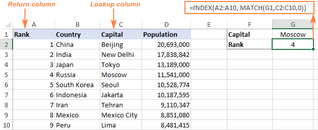
Tip. If you plan to use your INDEX MATCH formula for more than one cell, be sure to lock both ranges with absolute cell references (like $A$2:$A$10 and $C$2:4C$10) so they won't get distorted when copying the formula.
INDEX MATCH MATCH to search in rows and columns
In the above examples, we used INDEX MATCH as the replacement for classic VLOOKUP to return a value from a predefined one-column range. But what if you need to look up in multiple rows and columns? In other words, what if you want to perform the so-called matrix or two-way lookup?
This may sound tricky, but the formula is very similar to the basic Excel INDEX MATCH function, with just one difference. Guess what?
Simply, use two MATCH functions – one to get a row number and the other to get a column number. And I congratulate those of you who have guessed right :)
And now, please take a look at the below table and let's build an INDEX MATCH MATCH formula to find the population (in millions) in a given country for a given year.
With the target country in G1 (vlookup value) and the target year in G2 (hlookup value), the formula takes this shape:
=INDEX(B2:D11, MATCH(G1,A2:A11,0), MATCH(G2,B1:D1,0))
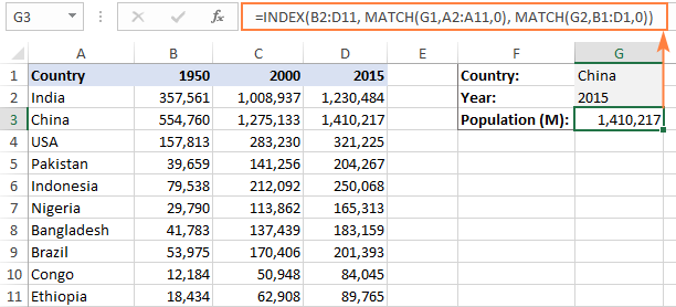
How this formula works
Whenever you need to understand a complex Excel formula, break it down into smaller parts and see what each individual function does:
MATCH(G1,A2:A11,0) – searches through A2:A11 for the value in cell G1 ("China") and returns its position, which is 2.
MATCH(G2,B1:D1,0)) – searches through B1:D1 to get the position of the value in cell G2 ("2015"), which is 3.
The above row and column numbers go to the corresponding arguments of the INDEX function:
INDEX(B2:D11, 2, 3)
As the result, you get a value at the intersection of the 2nd row and 3rd column in the range B2:D11, which is the value in cell D3. Easy? Yep!
Excel INDEX MATCH to look up multiple criteria
If you had a chance to read our Excel VLOOKUP tutorial, you have probably already tested a formula to Vlookup with multiple criteria. However, a significant limitation of that approach is the necessity to add a helper column. The good news is that Excel's INDEX MATCH function can look up with two or more criteria too, without modifying or restructuring your source data!
Here's the generic INDEX MATCH formula with multiple criteria:
Note. This is an array formula that must be completed with the Ctrl + Shift + Enter shortcut.
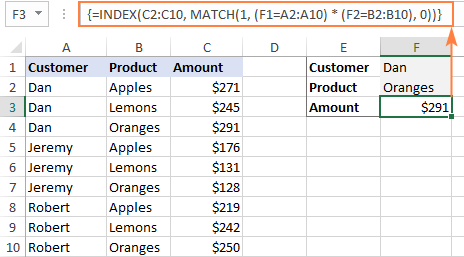
In the sample table below, supposing you want to find the amount based on 2 criteria, Customer and Product.
The following INDEX MATCH formula works a treat:
=INDEX(C2:C10, MATCH(1, (F1=A2:A10) * (F2=B2:B10), 0))
Where C2:C10 is the range to return a value from, F1 is criteria1, A2:A10 is the range to compare against criteria1, F2 is criteria 2, and B2:B10 is the range to compare against criteria2.
Remember to enter the formula correctly by pressing Ctrl + Shift + Enter, and Excel will automatically enclose it curly brackets as shown in the screenshot:
If you'd rather not use array formulas in your worksheets, add one more INDEX function to the formula and complete it with a usual Enter hit:
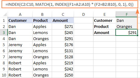
How these formulas work
The formulas use the same approach as the basic INDEX MATCH function that looks through a single column. To evaluate multiple criteria, you create two or more arrays of TRUE and FALSE values that represent matches and non-matches for each individual criterion, and then multiply the corresponding elements of these arrays. The multiplication operation converts TRUE and FALSE into 1 and 0, respectively, and produces an array where 1's correspond to rows that match all the criteria. The MATCH function with a lookup value of 1 finds the first "1" in the array and passes its position to INDEX, which returns a value in this row from the specified column.
The non-array formula relies on the ability of the INDEX function to handle arrays natively. The second INDEX is configured with 0 row_num so that it will pass the entire column array to MATCH.
That is a high-level explanation of the formula's logic. For full details, please see Excel INDEX MATCH with multiple criteria.
Excel INDEX MATCH with AVERAGE, MAX, MIN
Microsoft Excel has special functions to find a minimum, maximum and average value in a range. But what if you need to get a value from another cell that is associated with those values? In this case, use the MAX, MIN or AVERAGE function together with INDEX MATCH.
INDEX MATCH with MAX
To find the largest value in column D and return a value from column C in the same row, use this formula:
=INDEX(C2:C10, MATCH(MAX(D2:D10), D2:D10, 0))
INDEX MATCH with MIN
To locate the smallest value in column D and pull an associated value from column C, use this one:
=INDEX(C2:C10, MATCH(MIN(D2:D10), D2:D10, 0))
INDEX MATCH with AVERAGE
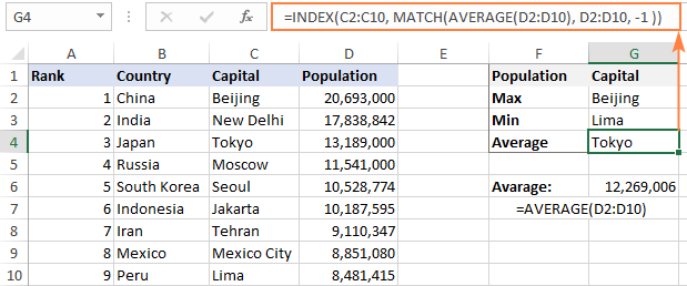
To work out the value closest to the average in D2:D10 and get a corresponding value from column C, this is the formula to use:
=INDEX(C2:C10, MATCH(AVERAGE(D2:D10), D2:D10, -1 ))
Depending on how your data is organized, supply either 1 or -1 to the third argument (match_type) of the MATCH function:
- If your lookup column (column D in our case) is sorted ascending, put 1. The formula will calculate the largest value that is less than or equal to the average value.
- If your lookup column is sorted descending, enter -1. The formula will compute the smallest value that is greater than or equal to the average value.
- If your lookup array contains a value exactly equal to the average, you can enter 0 for exact match. No sorting is required.
In our example, the populations in column D are sorted in descending order, so we use -1 for match type. As the result, we get "Tokyo" since its population (13,189,000) is the closest match that is greater than average (12,269,006).
You may be curious to know that VLOOKUP can perform such calculations too, but as an array formula: VLOOKUP with AVERAGE, MAX, MIN.
Using INDEX MATCH with IFNA / IFERROR
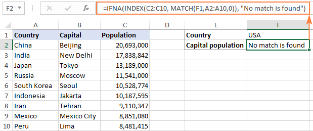
As you have probably noticed, if an INDEX MATCH formula in Excel cannot find a lookup value, it produces an #N/A error. If you wish to replace the standard error notation with something more meaningful, wrap your INDEX MATCH formula in the IFNA function. For example:
=IFNA(INDEX(C2:C10, MATCH(F1,A2:A10,0)), "No match is found")
And now, if someone inputs a lookup table that does not exist in the lookup range, the formula will explicitly inform the user that no match is found:
If you'd like to catch all errors, not only #N/A, use the IFERROR function instead of IFNA:
=IFERROR(INDEX(C2:C10, MATCH(F1,A2:A10,0)), "Oops, something went wrong!")
Please keep in mind that in many situations it might be unwise to disguise all errors because they alert you about possible faults in your formula.
That's how to use INDEX and MATCH in Excel. I hope our formula examples will prove helpful for you and look forward to seeing you on our blog next week!
Practice workbook for download
Excel INDEX MATCH examples (.xlsx file)
 by
by
600 comments
Is there a way to do a reverse index match? I have a calendar set up for appointments times by client name based on a weekly calendar grid. My software will give me a list of clients by date and time and I would like to populate the calendar without having to do it manually. Is there anyway to do this? Vlookup will do it by day, but not by time.
Hello, I am interested in the posibility I see in your Merge Duplicates wizard. However, it appears this may only be designed for finding duplicates within a column. Is there a tool which can merge duplicates within a ROW, and return the column headers as the output? Specifically, I would like to find all the zero cells in a row, ignore the non-zero cells, and compile a list of column headers for the zeros in each row.
hi ablebits team, please help with a formula that will compare multiple rows with multiple columns and match data of the same pattern.
table 1 table 2
a b c d a b c d e
6 13 35 60 5 6 35 39 60
i will really appreciate your help.
thanks.
Goodmorning Ms. Lana,
I am from the philippines. and i am very glad reading your articles. I have learned many things.
Do you have a free course regarding excel formula?
Please reply.
Thank you and mabuhay!
Hi Renato,
Thank you for your kind words! Regrettably, we do not have any courses on Excel. Our blog articles is all that we have :)
Hi, Could you please help me with the below criteria,
Eg,
A In
B Out
C out
D In
E In
F Out
Now I want to get the result of above criteria separately Like In’s separate and Out seperate with the help of formula.
I like too much. Thanks
I have an excel sheet with 5 columns. And 40000 rows of data.
1st column has Id no
2nd Date
3rd Name of institution
4th Subject
5th Course
The solution i require is
The formula should search for identical Ids, then search for identical date within that id, identical institution within that date, idential subject within that institution and concancenate the courses in one cell for that institution.
Can this be done by an array or does it need to write a macro.
I dont know much about arrays and macros. Please help find solution for this.
Hello, Saj,
We have a ready-made solution for your task. You can quickly and easily merge courses for identical values in the first four columns on your sheet using our Merge Duplicates Wizard.
I'm trying to return a list of individuals scheduled to work nights on a specific date.
Sheet 2
From Sheet 1, the names in column 1 associated with an array of shift values (i.e. N, N1CB, N2CB, N1, N2, etc) found in the column associated with the date entered in cell A1 on Sheet 2.
Sheet 1
Column A: Names
Row 1: Date (starting 1/1 - 12/31)
B2:NJ54: Variety of values showing shift worked (D, N, D1, N2, etc)
DEAR
I ENTERED A FORMULA BUT SHOWN IN #
NOW WHAT DO IDO ?
i input the FORMULA OF A6,=INDEX('RM DETAILS'!$J$5:$J$4101,MATCH(1,INDEX(('RM DETAILS'!$F$5:$F$4101='LAST PRICE'!A7)*('RM DETAILS'!$I$5:$I$4101=MAX(IF('RM DETAILS'!$F$5:$F$4101='LAST PRICE'!A7,'RM DETAILS'!$I$5:$I$4101))),0),0)) BUT OUT IS SHOWN #N/A
NOW WHAT DO I DO ?
This is my first time on any forum...
I'm trying to create a formula :
"Spreadsheet 1" is where I'm trying to get my information.
"Spreadsheet 2" Cell C2, the formula should read, "Refer to Cell A1 "A", look in Spreadsheet 1, and put the values for MON in cell C2, do the same for cell C3 and so forth.
Spreadsheet 1 contains: Spreadsheet 2:
A B C A B C
1 A MON 10 1 A
2 A TUE 11 2 MON ______
3 A WED 12 3 TUE ______
4 B MON 20 4 WED ______
5 B TUE 21 5 B
6 B WED 22 6 MON ______
7 C MON 31 7 TUE ______
8 C TUE 32 8 WED ______
9 C WED 33 9 C
I tried copying the table but got the above result.
But the crux is the first amount is the result from the same sheet and the second amount is result from another sheet.
Hi,
I did find the Index/Match multiple criteria formula very good however I have an issue in using this formula in different sheets.
Table 1 = Lookup
Table 2 = To be populated table
I have used the formula to check two criteria - a. Employee number and b. Department name.
The first row in the Lookup table in the relevant filed contains zero and so when I apply the formula the entire field is populated with zero [as in the first row of the Lookup table. I guess that this is because of the fixed reference rule applying.
Can I have the formula without Fixed reference so that the like data reference will be picked correctly?
Given below is the sample data table:
Formula used - {=INDEX(Lookup,MATCH(1,([@[Emp no]]=Lookup[Emp no])*([@Dept]=Lookup[Department]),0),25)}
Emp no Dept Amount Amount from another
from same sheet sheet.Repeats first
value
1 Governance 38000 38000
1 Customer Service 27000 38000
2 IT 40000 38000
2 Environment Services 35000 38000
Thanks for the assistance.
Hello
I am looking for a formula which will find a value first [(say Stock Name) from a table where there are many stocks with day to day turnover values}and then sum or average the corresponding values [day to day turnover for a month]for that particular stock.
Say for example:
Stock Name 5/12/17 6/12/17 7//12/17 8/12/17 9/12/17
ABBANK 20 22 25 15 12
Brac Bank 35 38 40 80 70
In another sheet we want to fetch the sum and average values for Brac Bank..
Please suggest...
Hello,
For me to understand the problem better, please send me a small sample workbook with your source data and the result you expect to get to support@ablebits.com. Please don't worry if you have confidential information there, we never disclose the data we get from our customers and delete it as soon as the problem is resolved.
Please also don't forget to include the link to this comment into your email.
I'll look into your task and try to help.
I don't usually do this but I have to give you praise for this wonderful example. Thank you so much!
There are 3 shifts, Every shift needs change duty after a Week (Sunday) of the month through 24:00 hrs. as given below detail.
Date: Friday,01/12/2017
Shift:A 00:00 TO 08:00 hrs (Night-duty)
Shift:B 08:00 TO 16:00 hrs (Morning-duty)
Shift:C 16:00 TO 24:00 hrs (Evening-duty)
Date: Saturday,02/12/2017
Shift:A 00:00 TO 08:00 hrs (Night-duty)
Shift:B 08:00 TO 16:00 hrs (Morning-duty)
Shift:C 16:00 TO 24:00 hrs (Evening-duty)
Date: Sunday,03/12/2017
Shift:A 00:00 TO 08:00 hrs (Night-duty)
Shift:B 08:00 TO 16:00 hrs (Morning-duty)
Shift:C 16:00 TO 24:00 hrs (Evening-duty)
Date: Monday,04/12/2017 (Duty Shift would be Changed)
Shift:A 16:00 TO 24:00 hrs (Evening-duty)
Shift:B 00:00 TO 08:00 hrs (Night-duty)
Shift:C 08:00 TO 16:00 hrs (Morning-duty)
Please help me that how to set formula in excel that will show me Shifts: A, B or C will perform their duties on given date in 24:00 hrs.
May kindly please be helped me in this case. in advance I shall be very thankful for him/her.
Hello,
I'm afraid there's no easy way to solve your task with a formula. Using a VBA macro would be the best option here.
However, since we do not cover the programming area (VBA-related questions), I can advice you to try and look for the solution in VBA sections on mrexcel.com or excelforum.com.
Sorry I can't assist you better.
Hello,
I'm trying to pull information from one sheet to another.
Basically I have one sheet with the following information
Distributor_Company Product_Name Price
Now I want to create a sheet for each Distributor Company that looks at the first sheet and pulls all the Product_name it carries and price
I have created the formula and its working only for each currency tab but i'm unable to create the formula in consolidated file could you please help/advise me for the above.
Curr. Amt in loc.cur. LCurr Eff.ex.rate Formulae Currency Actual Rate Rate +10% Rate -10%
AUD -21,928.99 SEK 6.4573 IF(AND(L2>$T$2,L2$T$2,L3<$S$2),"YES", "No") AUD/SEK AUD 6.45 7.09 5.80
EUR -8,905.29 SEK 9.7415 YES CHF/SEK CHF 8.42 9.26 7.57
EUR -5,668.19 SEK 9.7415 YES CNY/SEK CNY 1.27 1.40 1.14
EUR -21,310.71 SEK 9.7535 YES DKK/SEK DKK 1.31 1.44 1.18
GBP -3,030.09 SEK 11.16096 No GBP/SEK GBP 11.03 12.13 9.93
GBP -11,536.34 SEK 11.11894 No JPY/SEK JPY 0.07 0.08 0.07
NZD -21,607.94 SEK 5.78294 No NOK/SEK NOK 1.03 1.13 0.93
NZD -3,559.39 SEK 5.78292 No NZD/SEK NZD 5.81 6.39 5.23
USD -14,824.97 SEK 8.39942 No USD/SEK USD 8.42 9.26 7.58
USD -14,824.97 SEK 8.39942 No CZK/SEK CZK 0.38 0.42 0.34
I have created the formula but for each currency tab but i'm unable to create the formula in consolidated file could you please help/advise me for the above.
Thanks,
Chandru
Hello, Chandru,
For me to understand the problem better, please send me a small sample workbook with your source data and the result you expect to get to support@ablebits.com. Please don't worry if you have confidential information there, we never disclose the data we get from our customers and delete it as soon as the problem is resolved.
Please also don't forget to include the link to this comment into your email.
I'll look into your task and try to help.
Dear Ms. Svetlana
I need FIRST CHARACTER TO BE NUMERIC(SINGLE DIGIT 1 TO 9) FOLLOWED BY A DASH SYMBOL AND ONLY TEXT CHARACTER FOLLOWED BY IT, AND TOTAL LENGTH TO BE 6, Kindly can you tell me how to use it in data Validation tool in excel 2016
Product Code Product name
1-ABZX XXXXXX
9-BTGH XXXXXX
8-RCTB
6-XYXT
0-ABCD
Hello- This formula doesn't seem to be working for me. Can you tell me what I'm doing wrong.
I have the following problem:
Sheet 1 contains the following data:
M N
Period Room
2 356
2 246
3 310
6 361
4 315
5 313
7 3
1 GYM-C
7 155
2 201
5 204
7 266
4 3
6 259
1 110
1 364
3 201
5 3
7 110
7 266
4 204
6 1
2 201
3 201
6 155
1 240
5 360
2 201
Sheet 5 contains the following data:
A B C
Room Wave Period
1 A 5
3 A 5
110 B 5
112 B 5
114 B 5
125 A 5
151 D 5
154 D 5
155 D 5
158 D 5
160 D 5
161 D 5
201 B 5
202 B 5
203 B 5
204 B 5
205 B 5
210 B 5
213 B 5
217 B 5
240 C 5
246 C 5
254 C 5
255 C 5
258 C 5
259 C 5
264 C 5
265 C 5
266 C 5
270 C 5
304 A 5
310 A 5
313 A 5
315 A 5
351 D 5
352 D 5
355 D 5
356 D 5
357 A 5
359 D 5
360 D 5
361 A 5
362 A 5
366 A 5
212A B 5
212B B 5
Aqua Out A 5
Gym-B D 5
HCC A 5
RCA C 5
I need a formula that will match columns M & N of Sheet1 with Columns A & C of sheet 5 and return Column B of Sheet 5 in Sheet 1 "IF" Period=5.
Svetlana,
Thank you so much for your very logical and understandable explanation of the Index and Match function. I had dabbled with it in the past but never really grasped it. Your tutorial made it very clear! I was having problems on a spreadsheet using VLOOKUP where is would not allow me to have more than 2800 rows. I was able to switch to Index/Match and it works perfectly. Thank You!!!!
Hello Svetlana,
Thanks much for all the instructions on index/match functions.
I am trying to index an array and find the value in Column B if the value in Column A match a certain text string ignoring all spaces and any characters other than letters or numbers. For example, the text string I am trying to match is K15 but the column A may have K15 shown as K15, K 15, K-15, K_15, or K _ 15 etc. How can I make the index/match functions consider K15, K 15, K-15, K_15 and K _ 15 as the same text string when it does the matching search?
Thanks much and really hope I can get some help with this question.
Drew
Dear Svetlana Cheusheva,
I am a demand planner.
I have a 3 types of milk but I want raise demand on average consumption on milks, which formula will be apply on this condition.
Regards,
Mehmood
Hi - I am wondering for this formula,
=MATCH($C$78,$A$1:$L$1,0)
This allows me to return the column # there is a match of the text in C78 in Row 1, from column A to L.
Is it possible to extend this to an area i.e. multiple rows, vs single row? I want to do 20 rows i.e. $A$1 to $L$20 for example.
If I want it to return a value I want to translate to for each of the column, how do I specify? Say if it's in column A, it should populate with "Apple", column B with "Orange" etc.
Thanks a lot in advance!
Hi, Mandy,
since MATCH works with either column or row, you need to use VBA code or a macro to solve your task.
But I'm afraid we won't be able to help you with that. Please ask around Mr. Excel forum for it.
I wish I could help you better.
=IFERROR(INDEX($K$1:$AA$1,MATCH("Z",K3:AA3)),"YTS")
In the above Index-Match function, I wanted to Index a value from K1:AA1 by Matching and finding the final text value from K3:AA3. But, I want to exclude cells T3:V3. If I use the following, I get result only upto K3:S3. Please suggest a solution.
=IFERROR(INDEX($K$1:$S$1,MATCH("Z",K3:S3)),INDEX($W$1:$AA$1,MATCH("z",W3:AA3),"YTS"))
Thank you so much for this article.
Is there a way to populate a result in a cell matching two columns, looking for a value in column A and populating the corresponding value from column B? For instance I have column A listing 1-90. In Column B I have a dollar amount. I want to have that dollar amount as the automatic result when the same number from column A is typed in another cell. I hope this makes sense! :-)
Hi,
I have one doubt in Index match function with multiple criteria. If we have more than one identical values in the main sheet, it will pull the first found value from the lookup table. Is there any solution?
I have one sheet having Invoice number, amount, Supplier name, Currency. And in the main sheet for different Invoice numbers, same combination of Supplier name, currency and amount is there.
Hello, I am new to Excel and needing to write some formula or vlookup to select the min and the max values of an array like this one:
1 9/8/2017 20:20 x y 16,015.00 16,017.00
1 9/8/2017 20:20 x y 16,055.00 16,057.00
1 9/8/2017 20:20 x y 16,095.00 16,097.00
1 9/8/2017 20:20 x y 16,135.00 16,137.00
2 9/9/2017 15:55 x y 15,815.00 15,817.00
2 9/9/2017 15:55 x y 15,855.00 15,857.00
2 9/9/2017 15:55 x y 15,895.00 15,897.00
2 9/9/2017 15:55 x y 15,935.00 15,937.00
2 9/9/2017 15:55 x y 15,975.00 15,977.00
3 9/10/2017 1:02 x y 15,615.00 15,617.00
3 9/10/2017 1:02 x y 15,655.00 15,657.00
3 9/10/2017 1:02 x y 15,695.00 15,697.00
3 9/10/2017 1:02 x y 15,735.00 15,737.00
3 9/10/2017 1:02 x y 15,775.00 15,777.00
4 9/13/2017 1:26 x y 15,415.00 15,417.00
4 9/13/2017 1:26 x y 15,455.00 15,457.00
4 9/13/2017 1:26 x y 15,495.00 15,497.00
4 9/13/2017 1:26 x y 15,535.00 15,537.00
4 9/13/2017 1:26 x y 15,575.00 15,577.00
Would need to extract the 16,015 and the 16,137 for the cells with a 1 on the first column then do repeat the same for column with value 2, 3, 4...
The values needed to be returned for column with a value of 2 would be 15,815 and 15,977, column with a value of 3 would need to return 15,615 and 15,777......
Thank you very much in advance
Ev
I’m having some difficulty figuring out how to utilize Excel’s reference functions to do horizontal and vertical lookups, where the task is to search for a particular value in a specified row, and return the text value in the header of that value’s column. It seems like a combination of Index & Match would be desired, but I can't figure out a workable syntax that doesn't produce errors.
For example
Column A contains record ID’s. (e.g. 101-200)
Columns B-F contain options (e.g. apples, oranges, pears, etc.)
Cell values contain a 1 for first choice, 2 for second choice, 3 for third choice, blanks for unranked options.
An example of the desired outcome is to lookup a particular id (which would be identified by cell reference or formula, not a fixed row #), find the value ranked 1 in that row (values will not be ordered), and return the name of the option associated with that rank. For example, lookup record 25, find rank 1, return oranges if oranges is the header of the column containing rank 1 for record 25.
Any help would be greatly appreciated. Thank You.
Hi there,
I have a question that I am hoping somebody here might be able to provide some insight. So thanks in advance.
I have a table of values (%'s) as outlined below:
| Decile 3 | Decile 4 | Decile 5
Metric X 25.72 - 28.72 28.73 - 30.38 30.39 - 31.52
Metric Y 18.96 - 24.69 24.70 - 35.23 35.24 - 45.87
Also, I have data(%'s) as follows:
Metric X: 100 / 400 = 25.00. Now, based on this score, this results in the 2nd decile, as referenced above. Assuming that I "freeze the denominator", how much would the numerator (100) have to increase in order to reach decile 5? It would be easy to do some simple algebra to calculate that number.
However, I am trying to come up with an automated way to calculate the number to increase the numerator to achieve a given decile.
*Please disregard "Metric Y" above, but note that I have many metrics with different decile ranges in this table.
I appreciate all input.
Thanks!
**Correction, a 25.00 would result in Decile 1 that is not shown. That is not key, but I wanted to explain since I just caught that mistake.
Hi,
Really need your help.
Trying to create an excel spreadsheet that will help with costing for a construction project.
Column A: Area of task
Column B: Task
Column C: Cost code
I want to match the area and task and for the cell to output the cost code according to the lookup table. I tried to use the formula you have provided above but keep getting "#Value" - what am I doing wrong?
The values I want to match are part of a drop-down list. Is this my problem?
I think I figured out the problem - needed to press Crtl + Shift + Enter. How come we need to do that for this formula?
Is it possible to find answers that DON'T match? I have a list of people who have completed trainings. I can see which trainings they have completed, but I would like to see which ones they have not. I currently have the list of everyone who has completed certain courses, and I have a list of all required courses. I'd like to have a list of each name and the courses still required to be taken. Any suggestions would be helpful!
Hi there,
need help plz, am a beginner and trying to create a small template where I will be calculating price of goods plus GST applied. In description column I will write details of goods, now is there a way where I can apply a filter saying lets say description column is B. GST is applied on everything except food items. I have five items to list i.e.tea, coffee, sugar, creamer and Sweetener. so what formula can I try which will say if these 5 items GST will be 0 else it will be E*5%.
DESC QUANTITY UNIT PRICE SUB TOTAL GST
PILLOW 4 13 52 2.6
SUGAR 3 10 30 1.5
Hi,
I'm sorry, I'm afraid your task is not entirely clear for me. But from what I understand, I believe you may want to check out the following articles that may help you build the formulas:
COUNTIFS - to count the items.
IF - to return 0 or multiply by 5% depending on the COUNTIFS result.
I really hope you'll find those tutorials helpful.
Hi Svetlana, very interesting article. I was looking for how to do it but looking up for a value in a whole 2-dimensional range (matrix) instead of an array. The problem is that MATCH function only works with 1-dimension arrays. Any ideas?
Hi Manuel,
There are a few different ways to do 2-dimensional lookup in Excel. Please see this tutorial for full details: How to do two-way lookup in Excel
I have an array with column headings I am sorting on. Once I find the right column I need to copy all cells below to another location, where the original formula resides. Tried using INDEX and Match but come up with some crazy results. Can I use Index and Match to do this?
I have learned so much via your numerous invaluable articles. Your info has saved me so much time, especially with the more complex data compilation & analysis. I would gladly pay a subscription for all of this information. Thank you & thank you.
I'd like to take this opportunity to get a result from someone who has amazing skills in excel formula but to make everything simple. I had this little problem and this how it goes. Let say from column A1-A3 there is a duplicated info. Example: TB944009 (this is repeated thrice from A1-A3) Now, I have heavy table from my sheet that will certainly get the exact value that I want. My goal is to capture all infos that is equal from my look up value(Even if its different information). I use vlookup and it works out a bit, because every time I drag down my formulas it says N/A however, when you search it manually on the table you'll find it there. I tried to use $ sign(to limit the searching) for them to find all those information that I need. but it did not worked on my end. I hope that some one will share his/her knowledge so I can do my task easily. Thank you.
Hello:
After reading through this section there are some very creative solutions here. Unfortunately after a bunch of failed attempts I haven't quite figured out the correct method for solving mine, and request your assistance.
This problem involves the processing of a transaction log table of stock trade trades (buys and sells). The spreadsheet(s) contains 3 tables (in different sheets) , table 1 contains the transaction log, table 2 contains the symbols of each of the stocks in table 1, and table 3 contains the formulas for summarizing the data for each symbol collected from table 1.
In table 1 there can be many entries for each stock symbol and although most of the data I needed can be collected using Sumif(s). The ones that I am having a problem with is Min and Max.
Can you help with the formula for extracting the Min (or Min) values from the P&L column for each stock symbol using the symbols in table 2 please?
An example of table one is as follows:
A B C D
Symbol O_Price C_Price P&L
1 ABC $10.00 $11.00 $1.00
2 ABC $11.25 $11.85 $0.60
3 ABC $12.25 $11.85 ($0.40)
4 DEF
5 DEF etc.
6 DEF
7 DEF
8 etc.
Table 2
A
1 ABC
2 DEF
etc
Table 3 is the results table containing the summarized values, 1 row per symbol.
Thank you,
Cheech
thnx alot for explanation.
Hi there
tell me about the formula or function that to help me in tax if the tax little difference it not important
like the following example
ADELA 0.5 MCG tab ADELA TAB 0.5 MCG
ADVANT TAB 16 MG ADVANT TAB 16 MG
ADVANT 8 MG ADVANT TAB 8 MG
Hi!
I want to do a simple vlookup as normal. But I have 2 different "sets" I need to vlookup in...
Example:
Maine
Maine
Maine
Virginia
Virginia
Virginia
parts:
x, y & z available at both Maine and Virginia
I want to vlookup usage of X specifically in Virginia
Hi, I have an Excel workbook contains list of PlayStation players, so we merge them manually, then I want to do automatic check on those players name and check their score who win and it will also based on the first winner (maybe based on the time it was inputted) then the the formula should take the player to next level on the table.... The formula I was using before is if statement (=IF(C6>E6,B6,IF(E6>C6,F6))) so I discovered that some people don't play their game according to how we fix them, please what can I do to achieve this ...... The criteria I want to follow is this***check column c4:c200&e4:e200 the last inputted cell should and check the highest score, it should move the last player if the highest score is from column c or from column e
i would like to know if I will be able tp us e the match and index command to look at two rows one beneath each other to match if a number is the same between the two rows in each cell.
Once the match is found, can it then copy the two cells from each row to another cell
Thank you
Raj
A B C D
1 Name Date Issue Quantity
2 Sultan 15-03-16 Book 4
3 Rehman 16-5-16 Novel 3
4 Zakir 18-5-16 Pen 18
5 Sultan 19-5-16 Eraser 14
6 Zakir 20-5-16 Novel 8
I want that I just give a name in a cell and it show Complete Record in this sheet as like this.
Zakir
Zakir 18-5-16 Pen 18
Zakir 20-5-16 Novel 8
Wow, amazing articles!
How did you learn this all?
Thank you, Jenny! Just read a lot, practice a lot, and work with colleagues who know a lot more :)
hie help me on this one, which would I use to rank students using index match. One student is being dropped if they are sharing the same position. for example
Table 1
STUDENT NAME MARKS POSITION
MIKE RICHARD 560 1
CARLO JONES 555 2
RUTH TONEY 555 2
BRIAN JAMES 552 3
I want the formula to give me results as shown in table 1 above but instead I am having results as indicated below in table 2 with 1 student missing on the list
Table 2
STUDENT NAME MARKS POSITION
MIKE RICHARD 560 1
CARLO JONES 555 2
RUTH TONEY 555 2 - (missing on the list)
BRIAN JAMES 552 3
which formula should I use to have all students on the list even those sharing the same pos
Hi Svetlana,
I am trying to create a list of items not shipped out from our facility.
I have a workbook with 6 pages. Each pages represents one size of cylinders we are shipping. Each cylinder has numbers in numerical order listed down columns on the page.
Example:
RJ001
RJ002
RJ003
etc.
Each row of the cylinders has information like customers name, date ordered, order number, etc.
One column in the row I enter the "date shipped". I am struggling to create a summary page that will list ALL cylinders from ALL pages that has no "date shipped" filled in. I am just looking to list the cylinder numbers on the summary page which has the "date Shipped" column not filled in. Then when I fill it in, it will be removed from the list. Am I looking at the right formula for this or am I aimlessly struggling for nothing? Any help would be appreciated. :)