Dive into the Excel comparison: XLOOKUP vs INDEX MATCH. Curious about which formula reigns supreme in speed and efficiency? Uncover the secrets, discover the pros and cons, and choose the best formula for your specific needs!
One of the most common tasks in Excel is to look up values in a table based on some criteria. For example, you might want to find the price of a product, the name of a customer, or the sales amount for a given month. In the past, Excel users relied on the VLOOKUP function for this job. However, VLOOKUP had its fair share of limitations, leading savvy Excel enthusiasts to craft a more resilient solution using the INDEX MATCH combination. Now, with the advent of newer versions, we have the XLOOKUP function - a more powerful and versatile successor of VLOOKUP. This begs the question: does XLOOKUP not only outshine its predecessor but also surpass the tried-and-true INDEX MATCH combination? Let's delve into the features and nuances of these functions to find out.
XLOOKUP vs INDEX MATCH - syntax comparison
First things first, let's break down the syntax of these formulas and understand how they operate within Excel.
INDEX MATCH formula – the classic approach
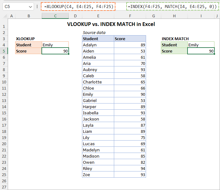
The INDEX and MATCH combination has stood the test of time as a classic method for various lookups in Excel. The syntax is as follows:
Here, the MATCH function determines the relative position of the lookup value in the lookup column, while INDEX retrieves the corresponding value from the return column at that position. The third argument of MATCH (match_type) set to 0 ensures an exact match, which is typically the desired behavior.
While this formula involves two separate functions, it provides great flexibility in handling various lookup scenarios.
For more information, see INDEX & MATCH formula in Excel.
INDEX XMATCH formula – improved version
A modernized alternative to MATCH, the XMATCH function was introduced concurrently with XLOOKUP and is only available in Excel 365 and Excel 2021. Here are the key improvements:
- Unlike MATCH, XMATCH defaults to an exact match, which aligns with most use cases.
- XMATCH does not require sorting the lookup array for an approximate match.
- In contrast to its predecessor, XMATCH can search in reverse order and perform a binary search optimized for speed. This behavior is controlled by the optional search_mode argument.
The syntax looks like this:
To put it briefly, INDEX XMATCH is a more advanced way of doing the same things as INDEX MATCH, which allows you to handle more complex and diverse lookup problems. In this tutorial, we will consider these formulas as essentially interchangeable, recognizing that each has its strengths and may be preferred in different contexts.
XLOOKUP function - the modern solution
The XLOOKUP function, often called the "killer" of VLOOKUP, represents a modern approach to lookup operations. It is only available for Office 365 subscribers and Excel 2021 users, offering a powerful alternative. The syntax for XLOOKUP is as follows:
Overcoming many limitations of VLOOKUP, XLOOKUP can handle a wide variety of scenarios, including left lookups, horizontal and vertical lookups, two-way lookups, and more. Its versatility makes it a go-to choice for users who want a comprehensive and effective lookup technique in the latest Excel versions.
For more details, see Excel XLOOKUP with formula examples.
Difference between XLOOKUP and INDEX MATCH
The way you choose to look up data in Excel can make a big difference in how smoothly your work goes. Let's explore the distinctions, so you can make the best choice for your specific requirements and the kind of data you're working with.
Here are some key differences to consider:
Compatibility. The INDEX MATCH formula works well in any version of Excel, making it a reliable and widely used option. The XLOOKUP function is only available for Excel 365 and Excel 2021 users; it is not backward compatible with older versions.
Flexibility. Both formulas can handle various lookup scenarios, such as vertical or horizontal lookups, left lookups, exact or approximate matches, multiple criteria, nested lookups, and more. They are both very resilient and robust tools for data retrieval.
Numeric index vs. return range. INDEX MATCH relies on the numeric index that represents the positions of the values you want to look up and return. The MATCH function finds the position of the lookup value, and INDEX returns the value at that position. This numeric index can be easily manipulated for various purposes, for example, to return values from different columns in your data. On the other hand, XLOOKUP operates on the return array reference, which is another way to do similar things.
Matching. The traditional INDEX MATCH formula can find exact matches in any dataset as well as approximate matches (closest smaller or closest larger) but only if your data is sorted. XLOOKUP and INDEX XMATCH can do any matching on unsorted data, thanks to the inherent features.
Reverse search. While INDEX MATCH can only look up from the beginning to the end, both XLOOKUP and INDEX + XMATCH can search in both directions: from first to last and from last to first.
Binary search. Another advantage of XLOOKUP and INDEX XMATCH is that they can be configured to use binary search, which is very fast and efficient for sorted data. Binary search works by dividing the range in half and checking if the value is in the left or right part. Then it repeats the process until it finds the value or reaches the end. This way, it can search through large amounts of data very quickly.
Handling errors. The INDEX MATCH combo does not have a built-in feature to handle errors. If the formula cannot find a lookup value, it will show #N/A. On the other hand, XLOOKUP has an extra argument (if_not_found) that lets you customize the response when there is no match. You can provide a certain value, display a friendly message, or even execute another formula.
How to use XLOOKUP instead of INDEX MATCH
And now, let's discuss practical examples to see how XLOOKUP can replace the old-fashioned INDEX MATCH formula to resolve various lookup problems in Excel.
Basic formula
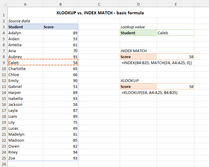
To illustrate the transition, let's consider a typical example where you have a list of student names in one column and their corresponding exam scores in another. In this scenario, you aim to retrieve the score for a particular student, say, in cell E4.
The INDEX MATCH formula for this task would look like this:
=INDEX(B4:B25, MATCH(E4, A4:A25, 0))
XLOOKUP provides an equally straightforward solution - just supply the required lookup value, lookup range and return range:
=XLOOKUP(E4, A4:A25, B4:B25)
As you can see in the screenshot, both formulas achieve the same result:
Left lookup
As you probably know, one of the greatest limitations of VLOOKUP is its inability to return values from columns located to the left of the lookup column.
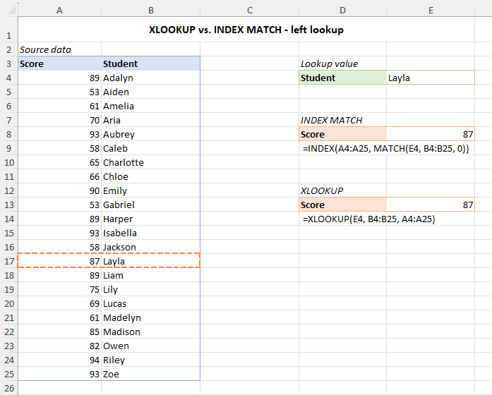
Both XLOOKUP and INDEX MATCH excel in handling left lookup tasks, providing a solution that VLOOKUP lacks. Here's how you can perform a left lookup with each method:
=INDEX(A4:A25, MATCH(E4, B4:B25, 0))
=XLOOKUP(E4, B4:B25, A4:A25)
Both formulas search for the specified value (E4) in column B and return the corresponding value from column A.
Horizontal lookup
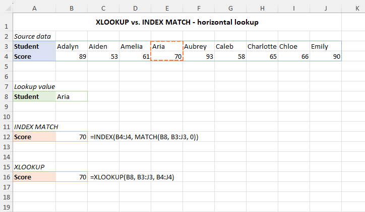
In older versions of Excel, the HLOOKUP function was specifically designed for searching horizontally in rows. The good news is that both XLOOKUP and INDEX MATCH are equally adept at performing horizontal lookups. To achieve this, you simply need to orient your lookup and return arrays in rows instead of columns.
=INDEX(B4:J4, MATCH(B8, B3:J3, 0))
=XLOOKUP(B8, B3:J3, B4:J4)
Handling entire columns and rows
When setting up real worksheets, it's common for users to refer to entire columns or rows in their formulas to account for potential data additions in the future. Both XLOOKUP and INDEX MATCH readily support this approach. For example:
=INDEX(A:A, MATCH(E4, B:B, 0))
=XLOOKUP(E4, B:B, A:A)
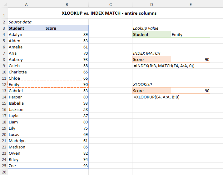
A word of warning for those who want to use this method: referencing whole columns or rows forces Excel to process very large arrays. This can affect performance and slow down your worksheets. You should always think about how this might impact calculation speed and try to limit your data ranges if performance is an issue.
Search in reverse order
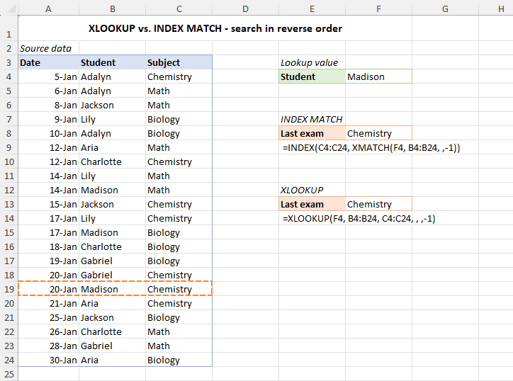
In scenarios where you need to search your data from the end to the beginning (bottom-to-top for vertical lookups or right-to-left for horizontal lookups) either XLOOKUP or INDEX XMATCH can help. It's worth noting that the MATCH function lacks this feature and cannot be applied in such situations.
To search last to first with XLOOKUP, you set the optional search_mode argument to -1:
=XLOOKUP(F4, B4:B24, C4:C24, , ,-1)
Similarly, for a reverse search using INDEX XMATCH:
=INDEX(C4:C24, XMATCH(F4, B4:B24, ,-1))
Two-way lookup
A two-way lookup, also known as “matrix” or “2-dimensional lookup”, is a technique that finds a value at the intersection of a specific row and column. The INDEX MATCH combo is well suited for this kind of lookup as INDEX can target both the row and column numbers, and you can employ two different MATCH functions for this purpose.
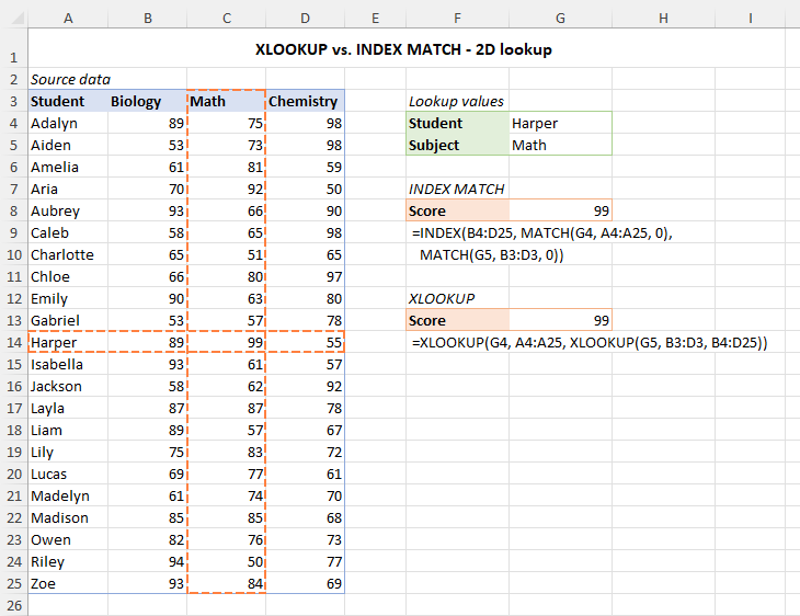
For instance, to get the score of a certain student in a particular subject, you can use this formula:
=INDEX(B4:D25, MATCH(G4, A4:A25, 0), MATCH(G5, B3:D3, 0))
Now, when it comes to a 2D lookup with XLOOKUP, it gets a bit more complex because it's primarily designed for a single lookup array. To handle both columns and rows simultaneously, you nest one XLOOKUP function inside another. The inner function looks for its value and returns a column or row of related data. This array then becomes the return_array for the outer function. Here's how it looks:
=XLOOKUP(G4, A4:A25, XLOOKUP(G5, B3:D3, B4:D25))
For more formula examples, please see How to do two-way lookup in Excel.
Multiple criteria lookup
The structure of both formulas allows for a fairly easy application of multiple criteria. The general approach is as follows: first, you test each condition individually, generating temporary lookup arrays of TRUE and FALSE values. Next, multiply the elements of these arrays to create a unified lookup array, where 1 represents a match and 0 represents no match. And then, you set the lookup_value to 1 to retrieve the first found match.
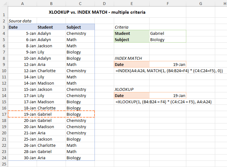
For example, to pull the date of a given exam (criteria1 – F5) for a particular student (criteria2 – F4), the formulas would go as follows:
=INDEX(A4:A24, MATCH(1, (B4:B24=F4) * (C4:C24=F5), 0))
=XLOOKUP(1, (B4:B24 = F4) * (C4:C24 = F5), A4:A24)
In Excel 2019 and earlier versions that do not support dynamic arrays, you need to enter INDEX MATCH as an array formula by pressing the Ctrl + Shift + Enter keys together. Otherwise, it will not work correctly. The non-array INDEX MATCH with multiple conditions formula also exists but has a slightly more complex syntax.
For in-depth understanding and practical examples, please refer to the following tutorials:
Return values from multiple columns
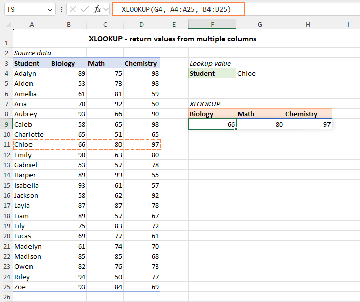
With XLOOKUP, getting information from multiple neighboring columns is a breeze, as long as those columns are adjacent to each other. Just choose the range that includes all the columns you need and serve it as the return array.
For instance, this is how you can retrieve the exam results from columns B, C, and D for a certain student in cell G4:
=XLOOKUP(G4, A4:A25, B4:D25)
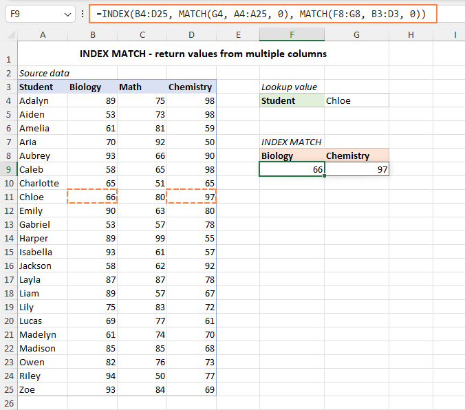
The INDEX MATCH duo goes a bit further by pulling data from any columns, even those that aren't next to each other:
=INDEX(B4:D25, MATCH(G4, A4:A25, 0), MATCH(F8:G8, B3:D3, 0))
In simple terms, this formula utilizes a 2-dimensional INDEX MATCH approach. The first MATCH finds the right row number for the student name in G4, and the second MATCH figures out the column numbers for the subjects in F8:G8.
Note that in Excel 2019 and older, this only works as an CSE array formula (requires pressing Ctrl + Shift + Enter to calculate correctly).
=XLOOKUP(G4, A4:A25, FILTER(B4:D25, {1,0,1}))
Handling missing values
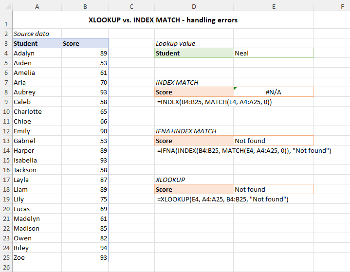
When a specified value is not found, the basic form of the INDEX and MATCH formula returns an #N/A error. However, you can mitigate this issue by wrapping the formula in the IFERROR or IFNA function and providing a custom message.
For instance, to replace an #N/A error with your own text, you can use INDEX MATCH together with IFNA:
=IFNA(INDEX(B4:B25, MATCH(E4, A4:A25, 0)), "Not found")
Alternatively, include your message in the 4th argument of XLOOKUP like this:
=XLOOKUP(E4, A4:A25, B4:B25, "Not found")
Both formulas achieve the same result, allowing you to handle missing values gracefully.
Which is better: XLOOKUP or INDEX MATCH?
How do you choose between XLOOKUP and INDEX MATCH in Excel? Determining the more appropriate method is based on several factors, such as:
- Excel version. If you have Excel 2021 or Office 365, you can use XLOOKUP. Otherwise, you have to rely on INDEX MATCH.
- Formula complexity. XLOOKUP has a simpler structure with fewer arguments. INDEX MATCH Involves more arguments due to its combination of two separate functions.
- Formula performance. XLOOKUP can perform faster than INDEX MATCH in some cases, especially if you use the binary search mode. However, INDEX MATCH can also be optimized by using Excel tables or dynamic arrays.
- Formula flexibility. Both formulas are versatile, capable of handling various lookup scenarios. However, adjustments may vary depending on the specific task.
- Formula readability. XLOOKUP has a more intuitive syntax and can be easier to understand and debug. INDEX MATCH has a more complex syntax and can be harder to follow and troubleshoot.
So, which is better? It depends on what you want to achieve and how you like to work. XLOOKUP is a modern option with a wide range of useful features, making it a good choice for many situations. However, INDEX MATCH is an enduring solution that has been used for decades in millions of worksheets, and some users may prefer it for its familiarity or extra control over the lookup functions.
Is INDEX MATCH faster than XLOOKUP?
This is a frequent inquiry among Excel users aiming to optimize their formulas and reduce calculation time. There is no simple answer, as it hinges on several variables such as the amount of data, the complexity of the criteria, and the version of Excel you are using.
In general, XLOOKUP is faster than INDEX MATCH for simple lookups, but INDEX MATCH can be faster for more advanced scenarios. Here are the key considerations to guide your choice:
Use XLOOKUP if:
- You are working with Excel 365 or 2021.
- You only need to look up a single value based on one criterion in a relatively small dataset.
- If you are working with sorted data where binary search is applicable.
Use INDEX MATCH if:
- You are using Excel 2019 or older.
- You are dealing with a substantial dataset.
- You need to perform lookups for multiple values based on multiple criteria.
For a comprehensive review of the fastest Vlookup methods in Excel, refer to the above-linked article, where we conducted in-depth research on this topic. It will show you some surprising findings and unveil some unexpected insights :)
Can XLOOKUP replace INDEX MATCH?
One of the most common questions that often arises in Excel discussions is whether the modern XLOOKUP function can effectively replace the longstanding INDEX MATCH combination. While both methods come with distinct advantages and limitations, the decision isn't a clear-cut one.
The key benefits of XLOOKUP are:
- It is simpler and shorter to write than INDEX MATCH.
- It can perform lookups in any direction: top-to-bottom, bottom-to-top, left-to-right as well as right-to-left.
- It can do both exact and approximate matches in any dataset, whereas INDEX MATCH is limited to approximate matches in sorted data.
- It can handle dynamic arrays and spill results to multiple cells.
- It can natively handle errors caused by missing values.
Some of the drawbacks of XLOOKUP are:
- It is not compatible with older versions of Excel 2019 and lower.
- It may not be as flexible as INDEX MATCH for some scenarios, such as returning values from non-contiguous columns.
- It may not work well with large data sets or volatile formulas.
In essence, XLOOKUP can indeed replace INDEX MATCH in many cases, but not all. The choice depends on Excel version compatibility, the complexity of your data, and personal preference.
XLOOKUP vs. INDEX MATCH - summary table
The below table provides a short summary of how XLOOKUP and INDEX MATCH differ in their functionality, benefits, and limitations.
| Feature | XLOOKUP | INDEX MATCH |
|---|---|---|
| Availability | Excel 2021, Excel 365, Excel for the web | All versions |
| Exact match | Yes | Yes |
| Approximate matching | Yes | INDEX MATCH – only on sorted data
INDEX XMATCH – on unsorted data |
| Wildcard search | Yes | Yes |
| Binary search | Yes | INDEX MATCH – no
INDEX XMATCH – yes |
| Lookup column needs to be sorted | For binary search | INDEX MATCH - for approximate match
INDEX XMATCH - for binary match |
| Vertical lookup | Yes | Yes |
| Horizontal lookup | Yes | Yes |
| Left lookup | Yes | Yes |
| Return entire rows or columns | Yes | Yes |
| Search in reverse order | Yes | INDEX MATCH – no
INDEX XMATCH – yes |
| Multiple criteria | Yes | Yes |
| Return values from multiple columns | Yes (adjacent columns) | Yes (any columns) |
| Built-in error handling | Yes | No |
In conclusion, both XLOOKUP and INDEX MATCH are powerful and convenient functions for performing various lookup tasks in Excel. Depending on your situation, you may prefer one over the other. However, it is always good to know both methods and how to use them effectively. Ultimately, the choice is yours.
Practice workbook for download
XLOOKUP vs. INDEX MATCH - examples (.xlsx file)
 by
by
2 comments
Hello,
So I have an inventory list of serial numbers on a spreadsheet for items that I have located at a depot maintenance facility, there are roughly 200. I have a second spreadsheet that is the master list that contains all the information by serial number for every item that was ever made for this same part number, there are almost 5000 items.
Is there a way to have excel search the master list by the SN's given on the inventory list from the depot facility, and have it return certain information from it such as "date of manufacture" and "recertification due date" etc.?
I am looking for a simple way of doing this instead of going 1 by 1 and line by line and just copying and pasting.
Thanks!
Hi! To search by SN and extract data from the master list, you can use one of the following instructions: Excel VLOOKUP function tutorial with formula examples or Excel INDEX MATCH vs. VLOOKUP or Excel XLOOKUP function with formula examples.
Create links to the master list using these instructions: Excel reference to another sheet or workbook (external reference).