The tutorial explains how to split cells in Excel using formulas and the Split Text feature. You will learn how to separate text by comma, space or any other delimiter, and how to split strings into text and numbers.
Splitting text from one cell into several cells is the task all Excel users are dealing with once in a while. In one of our earlier articles, we discussed how to split cells in Excel using the Text to Column feature and Flash Fill. Today, we are going to take an in-depth look at how you can split strings using formulas and the Split Text tool.
How to split text in Excel using formulas
To split string in Excel, you generally use the LEFT, RIGHT or MID function in combination with either FIND or SEARCH. At first sight, some of the formulas might look complex, but the logic is in fact quite simple, and the following examples will give you some clues.
Split string by comma, semicolon, slash, dash or other delimiter
When splitting cells in Excel, the key is to locate the position of the delimiter within the text string. Depending on your task, this can be done by using either case-insensitive SEARCH or case-sensitive FIND. Once you have the delimiter's position, use the RIGHT, LEFT or MID function to extract the corresponding part of the text string. For better understanding, let's consider the following example.
Supposing you have a list of SKUs of the Item-Color-Size pattern, and you want to split the column into 3 separate columns:
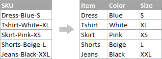
- To extract the item name (all characters before the 1st hyphen), insert the following formula in B2, and then copy it down the column:
=LEFT(A2, SEARCH("-",A2,1)-1)In this formula, SEARCH determines the position of the 1st hyphen ("-") in the string, and the LEFT function extracts all the characters left to it (you subtract 1 from the hyphen's position because you don't want to extract the hyphen itself).
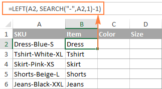
- To extract the color (all characters between the 1st and 2nd hyphens), enter the following formula in C2, and then copy it down to other cells:
=MID(A2, SEARCH("-",A2) + 1, SEARCH("-",A2,SEARCH("-",A2)+1) - SEARCH("-",A2) - 1)
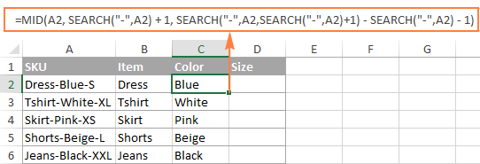
In this formula, we are using the Excel MID function to extract text from A2.
The starting position and the number of characters to be extracted are calculated with the help of 4 different SEARCH functions:
- Start number is the position of the first hyphen +1:
SEARCH("-",A2) + 1 - Number of characters to extract: the difference between the position of the 2nd hyphen and the 1st hyphen, minus 1:
SEARCH("-", A2, SEARCH("-",A2)+1) - SEARCH("-",A2) -1
- Start number is the position of the first hyphen +1:
- To extract the size (all characters after the 3rd hyphen), enter the following formula in D2:
=RIGHT(A2,LEN(A2) - SEARCH("-", A2, SEARCH("-", A2) + 1))In this formula, the LEN function returns the total length of the string, from which you subtract the position of the 2nd hyphen. The difference is the number of characters after the 2nd hyphen, and the RIGHT function extracts them.
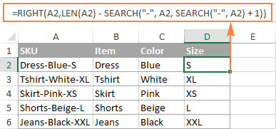
In a similar fashion, you can split column by any other character. All you have to do is to replace "-" with the required delimiter, for example space (" "), comma (","), slash ("/"), colon (";"), semicolon (";"), and so on.
Tip. In the above formulas, +1 and -1 correspond to the number of characters in the delimiter. In this example, it's a hyphen (1 character). If your delimiter consists of 2 characters, e.g. a comma and a space, then supply only the comma (",") to the SEARCH function, and use +2 and -2 instead of +1 and -1.
How to split string by line break in Excel
To split text by space, use formulas similar to the ones demonstrated in the previous example. The only difference is that you will need the CHAR function to supply the line break character since you cannot type it directly in the formula.
Supposing, the cells you want to split look similar to this:
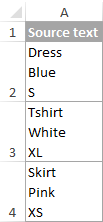
Take the formulas from the previous example and replace a hyphen ("-") with CHAR(10) where 10 is the ASCII code for Line feed.
- To extract the item name:
=LEFT(A2, SEARCH(CHAR(10),A2,1)-1) - To extract the color:
=MID(A2, SEARCH(CHAR(10),A2) + 1, SEARCH(CHAR(10),A2,SEARCH(CHAR(10),A2)+1) - SEARCH(CHAR(10),A2) - 1) - To extract the size:
=RIGHT(A2,LEN(A2) - SEARCH(CHAR(10), A2, SEARCH(CHAR(10), A2) + 1))
And this is how the result looks like:
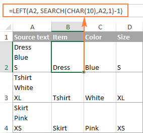
How to split text and numbers in Excel
To begin with, there is no universal solution that would work for all alphanumeric strings. Which formula to use depends on the particular string pattern. Below you will find the formulas for the two common scenarios.
Split string of 'text + number' pattern
Supposing, you have a column of strings with text and numbers combined, where a number always follows text. You want to break the original strings so that the text and numbers appear in separate cells, like this:
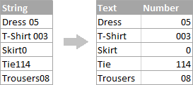
The result may be achieved in two different ways.
Method 1: Count digits and extract that many chars
The easiest way to split text string where number comes after text is this:
To extract numbers, you search the string for every possible number from 0 to 9, get the numbers total, and return that many characters from the end of the string.
With the original string in A2, the formula goes as follows:
=RIGHT(A2,SUM(LEN(A2) - LEN(SUBSTITUTE(A2, {"0","1","2","3","4","5","6","7","8","9"},""))))
To extract text, you calculate how many text characters the string contains by subtracting the number of extracted digits (C2) from the total length of the original string in A2. After that, you use the LEFT function to return that many characters from the beginning of the string.
=LEFT(A2,LEN(A2)-LEN(C2))
Where A2 is the original string, and C2 is the extracted number, as shown in the screenshot:
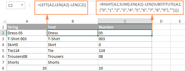
Method 2: Find out the position of the 1st digit in a string
An alternative solution would be using the following formula to determine the position of the first digit in the string:
=MIN(SEARCH({0,1,2,3,4,5,6,7,8,9},A2&"0123456789"))
Once the position of the first digit is found, you can split text and numbers by using very simple LEFT and RIGHT formulas.
To extract text:
=LEFT(A2, B2-1)
To extract number:
=RIGHT(A2, LEN(A2)-B2+1)
Where A2 is the original string, and B2 is the position of the first number.
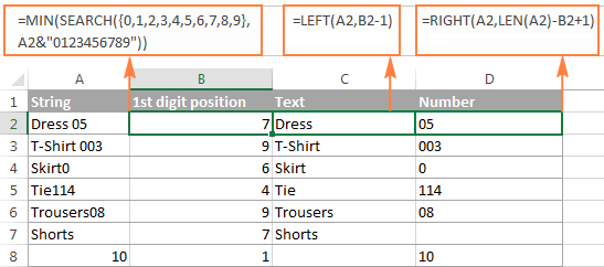
To get rid of the helper column holding the position of the first digit, you can embed the MIN formula into the LEFT and RIGHT functions:
Formula to extract text:
=LEFT(A2,MIN(SEARCH({0,1,2,3,4,5,6,7,8,9},A2&"0123456789"))-1)
Formula to extract numbers:
=RIGHT(A2,LEN(A2)-MIN(SEARCH({0,1,2,3,4,5,6,7,8,9},A2&"0123456789"))+1)
Split string of 'number + text' pattern
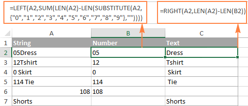
If you are splitting cells where text appears after number, you can extract numbers with the following formula:
=LEFT(A2, SUM(LEN(A2) - LEN(SUBSTITUTE(A2, {"0","1","2","3","4","5","6","7","8","9"}, ""))))
The formula is similar to the one discussed in the previous example, except that you use the LEFT function instead of RIGHT to get the number from the left side of the string.
Once you have the numbers, extract text by subtracting the number of digits from the total length of the original string:
=RIGHT(A2,LEN(A2)-LEN(B2))
Where A2 is the original string and B2 is the extracted number, as shown in the screenshot below:
Tip. To get number from any position in a text string, use either this formula or the Extract tool. Or you can create a custom function to split numbers and text into separate columns.
This is how you can split strings in Excel using different combinations of different functions. As you see, the formulas are far from obvious, so you may want to download the sample Excel Split Cells workbook to examine them closer.
If figuring out the arcane twists of Excel formulas is not your favorite occupation, you may like the visual method to split cells in Excel, which is demonstrated in the next part of this tutorial.
How to split cells in Excel with Split Text tool
An alternative way to split a column in Excel is using the Split Text feature included with our Ultimate Suite for Excel, which provides the following options:
To make things clearer, let's have a closer look at each option, one at a time.
Split cells by character
Choose this option whenever you want to split the cell contents at each occurrence of the specified character.
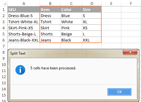
For this example, let's the take the strings of the Item-Color-Size pattern that we used in the first part of this tutorial. As you may remember, we separated them into 3 different columns using 3 different formulas. And here's how you can achieve the same result in 2 quick steps:
- Assuming you have Ultimate Suite installed, select the cells to split, and click the Split Text icon on the Ablebits Data tab.
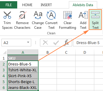
- The Split Text pane will open on the right side of your Excel window, and you do the following:
- Expand the Split by character group, and select one of the predefined delimiters or type any other character in the Custom box.
- Choose whether to split cells to columns or rows.
- Review the result under the Preview section, and click the Split button.
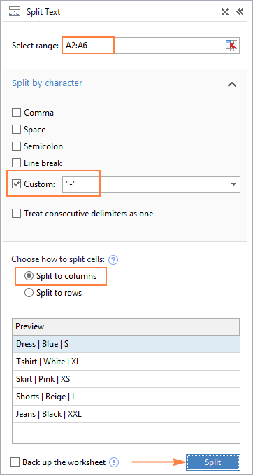
Tip. If there might be several successive delimiters in a cell (for example, more than one space character), select the Treat consecutive delimiters as one box.
Done! The task that required 3 formulas and 5 different functions now only takes a couple of seconds and a button click.
Split cells by string
This option lets you split strings using any combination of characters as a delimiter. Technically, you split a string into parts by using one or several different substrings as the boundaries of each part.
For example, to split a sentence by the conjunctions "and" and "or", expand the Split by strings group, and enter the delimiter strings, one per line:
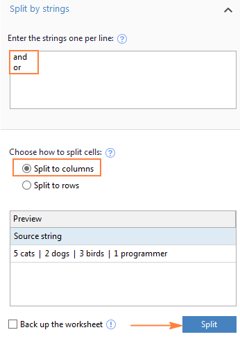
As the result, the source phrase is separated at each occurrence of each delimiter:

Tip. The characters "or" as well as "and" can often be part of words like "orange" or "Andalusia", so be sure to type a space before and after and and or to prevent splitting words.
And here another, real-life example. Supposing you've imported a column of dates from an external source, which look as follows:
5.1.2016 12:20
5.2.2016 14:50
This format is not conventional for Excel, and therefore none of the Date functions would recognize any of the date or time elements. To split day, month, year, hours and minutes into separate cells, enter the following characters in the Split by strings box:
- Dot (.) to separate day, month, and year
- Colon (:) to separate hours and minutes
- Space to separate date and time
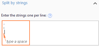
Hit the Split button, and you will immediately get the result:

Split cells by mask (pattern)
Separating a cell by mask means splitting a string based on a pattern.
This option comes in very handy when you need to split a list of homogeneous strings into some elements, or substrings. The complication is that the source text cannot be split at each occurrence of a given delimiter, only at some specific occurrence(s). The following example will make things easier to understand.
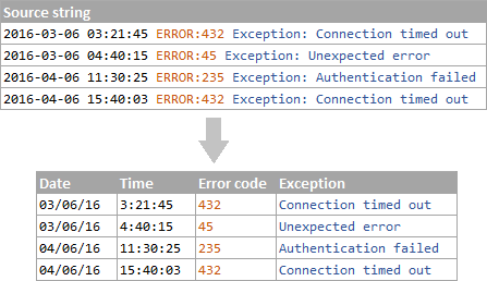
Supposing you have a list of strings extracted from some log file:

What you want is to have date and time, if any, error code and exception details in 3 separate columns. You cannot utilize a space as the delimiter because there are spaces between date and time, which should appear in one column, and there are spaces within the exception text, which should also appear in one column.
The solution is splitting a string by the following mask: *ERROR:*Exception:*
Where the asterisk (*) represents any number of characters.
The colons (:) are included in the delimiters because we don't want them to appear in the resulting cells.
And now, expand the Split by mask section on the Split Text pane, type the mask in the Enter delimiters box, and click Split:
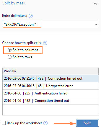
The result will look similar to this:

Note. Splitting string by mask is case-sensitive. So, be sure to type the characters in the mask exactly as they appear in the source strings.
A big advantage of this method is flexibility. For example, if all of the original strings have date and time values, and you want them to appear in different columns, use this mask:
* *ERROR:*Exception:*
Translated into plain English, the mask instructs the add-in to divide the original strings into 4 parts:
- All characters before the 1st space found within the string (date)
- Characters between the 1st space and the word ERROR: (time)
- Text between ERROR: and Exception: (error code)
- Everything that comes after Exception: (exception text)
I hope you liked this quick and straightforward way to split strings in Excel. If you are curious to give it a try, an evaluation version is available for download below. I thank you for reading and hope to see you on our blog next week!
Available downloads
Excel Split Cells formulas (.xlsx file)
Ultimate Suite 14-day fully-functional version (.exe file)
 by
by
306 comments
Hi
I would like to take a string of numbers in one cell and separate it by "-". The original data came from a string of columns, which I concat into one cell.
Orignal data:
705000 336 10 01 000 0000 35500
Used Concatenate for the result below
7050003361001000000035500
want it to be
705000-336-10-01-000-0000-335500
Hello Shamrock!
Please try the following formula:
=SUBSTITUTE(A1," ","-")
or
=SUBSTITUTE("705000 336 10 01 000 0000 35500"," ","-")
Hope you’ll find this information helpful.
Instead of concatenating the number and then splitting it back out ...
Use a1 & "-" & b1 & "-" & "c1 to concatenate with the -'s already in place.
Hello Sir,
I have data '1234 to 56478' and wanted add comma only for values using excel function and data should look like '1,234 to 55,678'
How do I do this?
Hello Santhosh!
If I understand your task correctly, the following formula should work for you:
=LEFT(A1,FIND(" ",A1,1)-4) & ","&MID(A1,FIND(" ",A1,1)-3, LEN(A1) - FIND(" ",A1,1)+1) & ","&RIGHT(A1,3)
I hope it’ll be helpful.
Thank you Alexander, It is working for the data which I had given as example...But comma needs to added for every thousands for example for data like '1020000 to 4080000' should be coming as '1,020,000 to 4,080,000' which is not coming now....and also I have the data like'0 to 1360000' and '1360000 +' where this formula is not working.
Can you help me out with this?
I have bunch of excel data which looks like:
1234 to 56478 (Given formula is working here)
0 to 2450000
1090000 to 4080000
1360000 +
1234 to 56478
Hello Santhosh!
Please use the following formula
=TEXT(LEFT(A1,FIND(" ",A1,1)-1),"#,##0") & MID(A1,FIND(" ",A1,1), FIND(" ",A1,FIND(" ",A1,1)+1) - FIND(" ",A1,1)+1)&TEXT(RIGHT(A1,LEN(A1) - FIND(" ",A1,FIND(" ",A1,1)+1)),"#,##0")
If there is anything else I can help you with, please let me know.
Dear madam,
you explain it in detail but i am unable to get the function =cocatenate(A1,",",B1) using text1 and text 2 for exporting it to autocad. please guide me
Your sincerly
Satya prakash tiwari
New Delhi
Hello!
Please specify what is the format of the file you're exporting in autocad (.csv/.txt/.exl). Maybe it'll help to conver all the functions into values beforehand. If you describe your task in more detail, I'll try to find a solution for you.
How can I remove http:// from a website string?
Hello Elaine!
Please use the following formula
=MID(A1,SEARCH("//",A1,1)+2,LEN(A1)-7)
We have a ready-made solution for your task. I'd recommend you to have a look at our Ablebits Data - Extract Text and Remove Characters.
This tool is available as a part of our Ultimate Suite for Excel that you can install in a trial mode and use for 30 days for free: https://www.ablebits.com/files/get.php?addin=xl-suite&f=free-trial
Dear Sir,
what is the formula of pick the number only.
Ex- Abhijeet Kumar Singh-7678154068 ASDC
only I have need of contact number
Thanks
I need a formula for to split:
1/03/2019 12:31:27 PM
to make it read
01/03/2019 in one column and 12:31 PM in another column
Thank you!
If your data is in A1, in B1 put =INT(A1). Format it as date short. In C1 put =A1-B1 and format it as Time
Saiph
Need formula for combine two decimal data.
Example format
data1 = 0x1000
data2 = 0x20
data3 = data1 | data2
data3 = 0x1020
2 20/02/20 10:18:11.762 18 225 115 239 35 176 1 0 0 219 0 10 3 143 0 0 23 41 143 62 52 11 197 3 33 217 28 0 4 0 6 101 1 7 14 13 195 2 153 20 23 0 1 14 0 0 5 40 28 12 82 12 215 3 3 255 249 0 0 0 0 205 12 140 36 56 10 246 3 1 0 0 0 0 205 228 71 41 181 12 249 2 252 31 20 0 0 0 255 5 66 24 46 157
From above string
I need to get 145th to 149th decimal value. How would i get it.
I have strings of numbers e.g S-N123-AB-FG. I wish to strip the number down to S-N123
Can anyone assist me please?
Best Regards
Ed
I've been using these page as a reference for over a year to help cleanup my website downloads. It has been very helpful. Thanks. QUESTION-
For the life of me, I can't figure out how to save my own formula and cut and paste it into my excel spreadsheets. Whenever I do, Excel rejects the formula; however, If I hand type it each time, it is fine. If I copy these formulas from your website and paste them into excel and manually change them to suite my needs, it's fine. Just trying to figure out how to make this easier on me. I'd like to set up a macro, but the formulas keep getting rejected unless I manually hand type them each time.... very time consuming. Below are how my formulas should read. Any ideas?
=LEFT(L2, SEARCH(“]”,L2,1)-1)
=MID(L2, SEARCH(“]”,L2) + 1, SEARCH(“]”,L2,SEARCH(“]”,L2)+1) - SEARCH(“]”,L2) - 1)
=RIGHT(L2,LEN(L2) - SEARCH(“]”, L2, SEARCH(“]”, L2) + 1))
I have to split 40k cells data
In this coloumn of 40 thousand cells, multiple rows contains data that is partially duplicate
Like
Fruit orange big
Fruit orange small
Fruit orange tiny
Vegetable tomoto
Vegetable potato
Dairy product organic milk
Dairy product organic cheese
Dairy product organic cream
The cell should split once the content of the cell changes
Hello I have been tasked with a project at work.
I am trying to convert the following
7' 9 3/16"
7 9/16"
7"
8 3/8"
8' 2 15/16"
8' 2 7/16"
some of these work using this formula:
LEFT(B34,FIND("'",B34)-1)*12+SUBSTITUTE(MID(B34,FIND("'",B34)+1,LEN(B34)),"""","")
some of them pop up with a VALUE Error, I presume because the format is wrong some are just inches some are just feet and some are feet and inches. I am trying to find the right formula to help solve this issue. I am sure I will need to add some IFERRORS, or something. I could really use all the help I can get.
Thanks in advanced!
Hi.... i have the data in B2 like this (CUROFF : OTHAKALMANDAPAM POLLACHI MAIN ROAD,CONTACT DETAILS. : MOB : 6379745419,OFFRES : NO 70 ANJENEYAR COLONY ONDIPUDUR COIMBATORE SOUTH,CONTACT DETAILS. : MOB : 9894144376,CURRES : 48 MANOJ NAGAR KALANGAL ROAD KANNAMPALAYAM,CONTACT DETAILS. : MOB : 6379745419,PERMNENT : 48 MANOJ NAGAR KALANGAL ROAD KANNAMPALAYAM,CONTACT DETAILS. : MOB : 6379745419).... i need to split cell based on "CUROFF:" in c2, "OFFRES :" in D2, "CURRES :" in E2, "PERMNENT :" in G2.... can you please help me on this..... thanx in advance
Please guys I need a very urgent help, I have a data set like
356897609864
376554333890
225657755443
26H676889378
............
............
This numbers are randomly generated using RANDBETWEEN formula.
I want to break it into 6 up and 6 down in the same cell
I Have data in a cell in this shape
32202-6536360-9
I need out put in other cells as one character in each cell
3
2
2
0
2
-
6
5
3
6
3
6
0
-
9
Is there any solution.
Faculty 9-Over-9 Program: Ahn, Charles H; (45212); GR100000 Payroll
-I am trying to separate the "Ahn, charles H" and input it into a different cell.
Thank you in advance for your help!!
A0b1C2D3E4F5G6H7I8J9K
ff5ff5s6s4sfd5
sfdfd4465ss4ss5
How to separate Numbers and alphabets
Hello,
I need to extract and put in different columns just the PO# (PO+digits) of the below array of strings. Sometimes it is separated by a "," or a " ". And the number of digit of a PO can Vary.
PurchOrd-PO7825,PurchOrd-PO8037,PurchOrd-PO8095 PurchOrd-PO7920,PurchOrd-PO8025 PurchOrd-PO7616,PurchOrd-PO7786,PurchOrd-PO7797.1,PurchOrd-PO7843,PurchOrd-PO7986
Result expected : PO7825 | PO8037|...| PO7797.1
You would be such a hero if you could help me on this :)
Thank you very much in advance (with or without answer!)
DATA 1
"Interscience Sdn Bhd
2, Jalan Sg. Kayu Ara 32/38
Berjaya Industrial Park
40460SHAH ALAM
SELANGOR"
=RIGHT(G2,LEN(G2)-SEARCH(CHAR(10), G2, SEARCH(CHAR(10), G2,SEARCH(CHAR(10), G2,SEARCH(CHAR(10), G2)+1)+1) + 1))
output: Selangor
Hi,
I want to split the below text:
INSP INSPIRIT ENERGY HOLDINGS PLC ORD 0.001P
To be:
First column: INSP
Second Column: INSPIRIT ENERGY HOLDINGS PLC ORD 0.001P
briefly, i want to split the text after the first space and the rest of the text to be added in the next column.
Thanks
How do you use the Albeits split function when your data is in separate lines (i.e. char(10) is the "demlimeter"? I have to split addresses and some may or may not have multiple lines of address.
Examples:
123 Main St
Bldg 5
Apt 19
123 Main St
Apt 10
123 Main St.
I was using the formulas at first but they only worked if all 3 lines existed.
Thanks, Laurie
If we have one cell that can say something like "24 hours, 72 hours, 1 week, 2 weeks, 4 weeks, 8 weeks, 12 weeks" (there can be many different possibilities in this cell), is there a way to display results in multiple cells of that same row, but instead of just displaying the words "24 hours", "1 week", etc, we need it to instead display an actual date in those multiple cells, each cell calculating the actual date based on another cell ("Start Date" field which is a date field), so one cell would display the date that is 24 hours after the Start Date, the next cell would display the date that is 72 hours after the Start Date, the next cell would display the date that is 1 week after the Start Date, and so forth and so on. I'm thinking this can either be calculated out before or after doing the text-to-columns thing? Ideally calculated out DURING the text-to-columns thing so it is done in one fell swoop. Does this make sense?
Please need your kind guidance to split this text into proper column.
A Thomas Hall III Hall Enterprises, Inc. 29075 Palos Verdes Dr E Rancho Palos Verdes, CA 90275-6405
A. Carol Brooks, CPL Independent 2504 Glenwood Cir Edmond, OK 73034-6487
A. Ray Davis, CPL Davis Land & Minerals, Inc. PO Box 79188 Houston, TX 77279-9188
A. Earl Irby Jr. Independent PO Box 428 Round Rock, TX 78680-0428
A. Frank Klam, CPL Independent 8309 Cedarbrake Dr Houston, TX 77055-4823
A. E. Martin CPL Retired PO Box 580 Oklahoma City, OK 73101-0580
A. Byron Pugh III, CPL Professional Energy Services, Inc. PO Box 820387 Houston, TX 77282-0387
A. Dale Anderson, CPL/ESA Anderson & Associates Inc. PO Box 701 Mount Vernon, IL 62864-0015
A. John Davis Holland & Hart LLP 222 S Main St Ste 2200 Salt Lake City, UT 84101-2194
A. Scott Fairbanks Summit Systems Consulting 241 N 4th St Unit 472 Grand Junction, CO 81502-5819
Hi, I created 4 additional columns to simplify the formula.
By locating unique idenifiers (spaces and the US MALE or US FEMALE) you then know the relative positions of the other data and can chop it out with ease.
Unless other text appears the FINDS are looking for a single Space.
Data is in A3
In B3: =FIND(" ",A3)
In C3: =FIND(" ",A3,B1+1)
In D3: =FIND(" ",A3,C1+1)
In E3: =IFERROR(FIND("US FEMALE ",A3)-11,FIND("US MALE ",A3)-11)
in F3 will be first name :=LEFT(A3,B3)
in G3 will be surname : =TRIM(MID(A3,B3,C3-B3))
in H3 will be email : =MID(A3,C3,D3-C3)
in I3 will be Address: =MID(A3,D3,E3-D3)
Hi,
I have a text file containing name, emails, address and many more its all 42 columns and doesn't have any headers and delimiters. I want the data in order as first name and last name in column and address in one column. I need a solution how to grab one records address data in one column as you see sample data that address is separated with spaces can you get me a solution . Here is the sample of my data.
4391 Grig Mcdaniil mail@hotmailcom 3619 N. Tiffany Drivi Beavercreek NY 75637 5046851665 US MALE 09/30/1959 178 182 AB+ Grig Mcdaniil Frank Blacker ATHENS IL 61516 US N.A NO YES NO NO N.A FR-DLI09-i3089 09/30/1959 $200.00 Grig Mcdaniil Pamela Toloza BaX_OlaCm-2441 09/30/1959 MALE Other VALIUM37.5 MG 90 $2.85 $171.00$20.00 $191.00
4392 Harold Davis mail@infinet 488 Wrins Nist Ct bay city FL 54311 5260805557 US MALE 10/17/1952 173 182 AB+ Harold Davis Owen K Ritter DENVERCA N.A US 9002005495 YES NO YES NO NO Yt_i7-Un-10375 10/17/1952 $250.00 Harold Davis Heidi Schultz BaX_OlacM-52110/17/1952 MALE Gas PHENTERMINE 37.5 MG 90 $1.90 $505.00$20.00 $525.00
Apologies. Failed to Reply, but posted the answer as a new question.(77)
Dear folks,
In many text files, I have a series 80 digits (0-9) in a row and multiple rows. I need to count the occurrences of each digit row-wise and column-wise. This can be done if I can split each digit into one column when I import from the text file. I can do this by painfully marking the delimit by Width for each character for 80 characters when I do the import. Is there any way to save this delimit method and use that method to import a file as I open each text file?
Thanks in advance to all of you,
Joe.
Hi Joe,
From what I can see, there doesn't seem to be a 'save delimiter' function.
There are definitely options though. For multiple text files a macro may be the easiest option.
Create an excel enabled macro workbook and put the macro in it. Save it.
Open the text file with NO formatting so you have x many rows with 80 characters all in column A
Run the macro.
Sub Convert80()
'
' CONVERT BLOCK OF 80 CHARACTERS TO 80 COLUMNS
'
Columns("A:A").Select
Selection.TextToColumns Destination:=Range("A1"), DataType:=xlFixedWidth, _
FieldInfo:=Array(Array(0, 1), Array(1, 1), Array(2, 1), Array(3, 1), Array(4, 1), Array _
(5, 1), Array(6, 1), Array(7, 1), Array(8, 1), Array(9, 1), Array(10, 1), Array(11, 1), Array _
(12, 1), Array(13, 1), Array(14, 1), Array(15, 1), Array(16, 1), Array(17, 1), Array(18, 1), _
Array(19, 1), Array(20, 1), Array(21, 1), Array(22, 1), Array(23, 1), Array(24, 1), Array( _
25, 1), Array(26, 1), Array(27, 1), Array(28, 1), Array(29, 1), Array(30, 1), Array(31, 1), _
Array(32, 1), Array(33, 1), Array(34, 1), Array(35, 1), Array(36, 1), Array(37, 1), Array( _
38, 1), Array(39, 1), Array(40, 1), Array(41, 1), Array(42, 1), Array(43, 1), Array(44, 1), _
Array(45, 1), Array(46, 1), Array(47, 1), Array(48, 1), Array(49, 1), Array(50, 1), Array( _
51, 1), Array(52, 1), Array(53, 1), Array(54, 1), Array(55, 1), Array(56, 1), Array(57, 1), _
Array(58, 1), Array(59, 1), Array(60, 1), Array(61, 1), Array(62, 1), Array(63, 1), Array( _
64, 1), Array(65, 1), Array(66, 1), Array(67, 1), Array(68, 1), Array(69, 1), Array(70, 1), _
Array(71, 1), Array(72, 1), Array(73, 1), Array(74, 1), Array(75, 1), Array(76, 1), Array( _
77, 1), Array(78, 1), Array(79, 1), Array(80, 1)), TrailingMinusNumbers:=True
Range("A1").Select
End Sub
I'm trying to get the text after the third "/" in a list of class names in the form:
MIL/MZ/AD/INT-B1-BLUE-29-10-19-Tue-W-F-10:00-13:00
With the formula below from the top of your thread I can get rid of MIL/MZ/ but I still need to get rid of AD/
=RIGHT(F2,LEN(F2) - SEARCH("/", F2, SEARCH("/", F2) + 1))
is giving me
AD/INT-B1-RED-23-09-19-M-W-Th-18:30-21:30
I tried playing and came up with:
=RIGHT(F2,LEN(F2) - SEARCH("/", F2, SEARCH("/", F2, SEARCH("/", F2) + 1)))
Which gives the same result as:
=RIGHT(F2,LEN(F2) - SEARCH("/", F2, SEARCH("/", F2) + 1))
I really don't understand the syntax so I've reached an impasse. If you are able to help I'd be grateful.
Thanks in anticipation.
You have the answer, just need to do another RIGHT command to get the characters to the right of the remaining '/' symbol.
=RIGHT(RIGHT(B2,LEN(B2)-(SEARCH("/",B2,SEARCH("/",B2)+1))),LEN(RIGHT(B2,LEN(B2)-(SEARCH("/",B2,SEARCH("/",B2)+1))))-SEARCH("/",RIGHT(B2,LEN(B2)-(SEARCH("/",B2,SEARCH("/",B2)+1)))))
Hi guys, I have a situation here as i need to split this one sentence into different columns IN EXCEL using a formula, as all words having spaces of different types.
RDH10265/2 12,00 PC OPTICAL TRANSCEIVER/SFP+ SM 10.3Gb/s 1.4
Thanks
Use Find & Replace and replace 2 spaces with 1 space over the whole column. Run it multiple times till no changes occur. Now you can run formula and split out columns on single spaces.
how will u split the below sting where there is only enter key
1 Unit Fodder Grass Bijankur-BB2 50 gm Rs. 335
1 Unit Fodder Grass Alamdar 51 1 kg Rs. 675
1 Unit Fodder Grass Bijankur-BB2 50 gm Rs. 335
1 Unit Fodder Grass Alamdar 51 1 kg Rs. 675
Depending on where you want to break the text you can use LEFT, RIGHT and MID string.
=LEFT(A1,FIND("Rs.",A1)-1) to trim off the price
=NUMBERVALUE(RIGHT(A1,LEN(A1)-FIND("Rs.",A1)-3)) to get the price
I have data in a column of cells similar to the following:
A, B, C
A
B, C
A, C
B
So now I want to filter the column by the data. However when I do this< my choices would be:
A, B, C
A
A, C
B
B, C
Where I really just want to filter by:
A
B
C
Should I separate the data by a different character to get this? Or is this something I need to dig further into to do in VB? Currently the data is entered into the cell using a drop down box, & then have some VB coded to have multi, non-repetitive selections that are separated by a comma. Thanks.
Another character or assigning a value seems the easiest. Like Binary. A=1 B=2 C=4.
Then a custom filter = selecting A will show all 1,3,5 and 7
Selecting B will show 2,3 and 6
Selecting C will show 4,5 and 6
How about
71200 Online Order Fees $376.12
to 3 columns.
Account Description Amount (with no dollar$)
in A1 : 71200 Online Order Fees $376.12
in B1 : =LEFT(A1,FIND(" ",A1)-1)
in C1 : =MID(A1,FIND(" ",A1)+1,FIND("$",A1)-FIND(" ",A1)-2)
in D1 : =NUMBERVALUE(RIGHT(A1,LEN(A1)-FIND("$",A1)))
This is assuming no one puts a $ in the text...
Source is like this...
P. Umesh, 123 ramesh, 34 p. M. Kavya, 10,55
Out put
P. Umesh 123
Ramesh 34
P.m.kavya 10
P. M. Kavya 55
Could plz me this problem...
Hi,
I have a question need for it answer by formulas to split according to dash all the contents of cell into separator in many cells beside each other as following example:
What I have in Cell A1:
Orange com - Emad Farag - Telephone bill - Month April 2019 - paid from cash
What I need in Cells C1, D1, E1, F1, G1
C1 D1 E1 F1 G1
Orange com Emad Farag Telephone bill Month April 2019 paid from cash
Thanks
Hi Emid, Is your problem solved or I can help you in solving the problem.
In an XL spread sheet - column "?" I'd like to split rows #25, 26, 27, 28, 29 & 30 BUT not add an additional column. These rows are situated partway down an XL spreadsheet and I cannot distrurb any columns or rows around this particular block.
Can this be accomplished?
E.g. - in each of the the cells:
Data 21
Data 22
Data 23 As per above, I'd like to keep the column and cells as is but have them "split" between "Data and the number value.
Appreciate any help you may have~!
Hi,
Please advise a formula for the below sample data
"Apple 8Ap #556-1337 Ali Avenue
Galaxy S823433 Eet, Av.
Google Pixel 2P.O. Box e446,Justo Av"
In the above lines i want to split Device and Address in two different cells using formulae.
For Eg: In Column 'A' we have "Apple 8Ap #556-1337 Ali Avenue", then using a formula i require
Device should be extracted in column B as "Apple 8"
Similarly, Address should be extracted in Column C "Ap #556-1337 Ali Avenue"
Note: I have 1000 different devices, where i should not entry any data manually.
Kindly help me with this.
Hi,
I have a huge data file in this text format:
"0009_000006-1","Camera Equipment"
"2/1/2018","2/28/2018","$39.83",""
"3/1/2018","3/31/2018","$39.83",""
"4/1/2018","4/30/2018","$39.83",""
"5/1/2018","5/31/2018","$39.83",""
"6/1/2018","6/30/2018","$39.83",""
"7/1/2018","7/31/2018","$39.83",""
"8/1/2018","8/31/2018","$39.83",""
"9/1/2018","9/30/2018","$39.83",""
"10/1/2018","10/31/2018","$39.83",""
"11/1/2018","11/30/2018","$39.88",""
"--------------------"
"Total for","2018",":","$398.35",""
"===================="
"--------------------"
"Totals for Asset:","0009_000006-1"
"Projection Grand Total:","$398.35"
"Pre-","Projection Grand Total:","$0.00"
"===================="
"0009_000025-1","34801 HP Elitebook 840G1"
"2/1/2018","2/28/2018","$42.10",""
"3/1/2018","3/31/2018","$42.10",""
"4/1/2018","4/30/2018","$42.10",""
"5/1/2018","5/31/2018","$42.10",""
"6/1/2018","6/30/2018","$42.10",""
"--------------------"
"Total for","2018",":","$210.50",""
"===================="
How can I convert this huge data file to excel format so I can create pivot table:
Asset ID Asset Class Begin Date End Date Amount
0009_000006-1 Camera Equipment 2/1/2018 2/28/2018 $39.83
0009_000006-1 Camera Equipment 3/1/2018 3/31/2018 $39.83
0009_000006-1 Camera Equipment 4/1/2018 4/30/2018 $39.83
0009_000006-1 Camera Equipment 5/1/2018 5/31/2018 $39.83
0009_000006-1 Camera Equipment 6/1/2018 6/30/2018 $39.83
0009_000006-1 Camera Equipment 7/1/2018 7/31/2018 $39.83
0009_000006-1 Camera Equipment 8/1/2018 8/31/2018 $39.83
0009_000006-1 Camera Equipment 9/1/2018 9/30/2018 $39.83
0009_000006-1 Camera Equipment 10/1/2018 10/31/2018 $39.83
0009_000006-1 Camera Equipment 11/1/2018 11/30/2018 $39.88
0009_000025-1 34801 HP Elitebook 840G1 2/1/2018 2/28/2018 $42.10
0009_000025-1 34801 HP Elitebook 840G1 3/1/2018 3/31/2018 $42.10
0009_000025-1 34801 HP Elitebook 840G1 4/1/2018 4/30/2018 $42.10
0009_000025-1 34801 HP Elitebook 840G1 5/1/2018 5/31/2018 $42.10
0009_000025-1 34801 HP Elitebook 840G1 6/1/2018 6/30/2018 $42.10
It would help me a deal if you can assist. Thank you!
Hi Lynn, is your problem solved or I can help you?
Hi there,
I want to split a text in one cell into different columns but can the text be rearranged in a specific order?
Cell A1 = Yellow/Magenta
Cell A2 - Magenta/Yellow
I would like Cell B1 = Yellow, C1 = Magenta, Cell B2 = Yellow and Cell C2 = Magenta
Is there a formula that can do this?
Thank you
Use a column specific formula
Assuming Data is in A1,A2 etc
In B1
=IFERROR(IF(FIND("Yellow",$A1)>0,"Yellow",""),"")
In C1
=IFERROR(IF(FIND("Magenta",$A1)>0,"Magenta",""),"")
In D1
=IFERROR(IF(FIND("next color",$A1)>0,"next color",""),"")
The iferror stops the formula failing and puts a blank if the color is not found. If it is found anywhere in the string then it will show.
The only problem you might have is putting in a "Light Yellow" as this will also flag as Yellow
Hi there,
I want to split text from a specific word. Would you please anyone share the formula.
The raw date are given below.
CLS1103 EIDF19 DUSTY BLUE
CLSMK09 EIDF19 60E MIDNIGH
What I want split from Eidf19. So cls1103 eidf19 is 1st column and 2nd column is dusty blue
I have a single column of text which I want to parse into various columns, but the delimiter is currently multiples of blank spaces in front of the text. Such as the data which should be in the first column has 5 blanks in front, the data which should be in the second has 10 blanks in front and the data which should be in the third column has 15 blank spaces in front of the text. Example of how this looks in the current single column:
Column1 text
Column2 text
Column3 text.
The amount of text may vary in each column, but the leading blank spaces are constant. Thanks for your help!
That didn't show up correctly, let me use _to emulate a blank space (but there are actually only spaces, no leading characters):
_____text column 1 info
__________text column 2 info
_______________text column 3 info
I hope that is more clear. Thanks.
data in A1.
These formulae take the data before the first 10 spaces as column 1, between 10 and 15 as column 2 and to the right of 15 spaces as column 3
B1 =TRIM(LEFT(A1,FIND(" ",A1)))
C1 =TRIM(MID(A1,FIND(" ",A1),FIND(" ",A1)-FIND(" ",A1)))
D1 =TRIM(RIGHT(A1,LEN(A1)-FIND(" ",A1)))
B1 =TRIM(LEFT(A1,FIND("10",A1)))
C1 =TRIM(MID(A1,FIND("10",A1),FIND("15",A1)-FIND("10",A1)))
D1 =TRIM(RIGHT(A1,LEN(A1)-FIND("15",A1)))
website took out my spaces.
numbers in the speechmarks are number of spaces.
=LEFT(TRIM(B34),FIND("~",SUBSTITUTE(B34," ","~",LEN(TRIM(B34))-LEN(SUBSTITUTE(TRIM(B34)," ",""))))-4)
Kindly define this formula.
Find the last space in the B34 string and take everything to the left of that, less 4 characters. The string must have spaces for this to work.
Is it just the way the syntax was created?
SEARCH("-",A2,SEARCH("-",A2)+1) - SEARCH("-",A2) - 1)
Hi Nathan,
To explain it better, let's have a look at the full formula:
=MID(A2, SEARCH("-", A2) + 1, SEARCH("-", A2, SEARCH("-",A2) +1) - SEARCH("-", A2) - 1)
1. Start_num argument: SEARCH("-",A2) + 1. It finds the position of the first character to extract; +1 is needed to start extraction beginning with the character that follows the first hyphen, not including the hyphen itself.
2. Num_chars argument (how many characters to extract): SEARCH("-", A2, SEARCH("-",A2) +1) - SEARCH("-", A2) - 1. To find the position of the 2nd hyphen, you put SEARCH("-",A2)+1) in the start_num of the first SEARCH function to tell it to start searching beginning with the character after the 1st hyphen (this way, you exclude the first hyphen from search). Then, you subtract the position of the 1st hyphen from the position of the 2nd hyphen to find how many characters are between them. But this number includes the 2nd hyphen, so you put -1 at the end to remove the 2nd hyphen from the returned substring.
In example #2 above, can you explain the +1 when finding the difference between the 2nd and 1st hyphens and how does the last search argument explains how the function understands how to extract all the characters between the two hyphens?
I have a full description of a part in one column and need to pull over no more then 35 characters. I need to do this at a "space" but not go over 35 characters on my limit. please help!
thanks!!
=LEFT(A1,FIND("☃",SUBSTITUTE(A1," ","☃",LEN(LEFT(A1,36))-LEN(SUBSTITUTE(LEFT(A1,36)," ","")))))
(Left(a1,36)) This trims the string to a maximum of 36 characters. 36 because if the 36th is a space then 35 chars will be returned and if not, then the break will come earlier in the string and less will be returned.
The statement LEN-LEN(substitute) finds the length of the string, and then the length with the spaces removed. This gives the number of spaces in the string.
The Substitute inside the Find statement then changes the last space to a snowman, and the Find returns that position in the string.
Finally the left statement cuts the string at that point and gives your value.
Hi , thanks a lot for this, but i have a big problem , it's only for 3 column, i am working as data entry and i have 10 column , hot to do this please help
Gemcitabine_pow_1000 mg_1 X 1V
Ranitidine_tab MR_150 mg_6 X 10T
Ranitidine_tab MR_300 mg_3 X 10T
Above text please separate from "_" (Only by formula) , Not by text to column
Please send me formula
I have the following data in one cell. i like to spit these data in different cells. is anybody can help?
1/15/2019 4320 610285062 1 30 0930 1143 88 167.75 14.26 $182.01
in Excel select the cell/column.
On the ribbon, choose Data tab, "Text to Columns" and select delimiter and then untick Tab and select Space
i have data in excel
A battery consists of (a) only one cell (b) only two cells (c) two or more cells (d) All of the above
Column A Column B Column C Column D Column E
i need to separate Data for example
1. Before (a) Column A
2. After (a) and Before (b) Column B
3. After (b) and Before (c) Column C
4. After (C) and Before (D) Column D
5. After (D) Column E
pls help
I have a text string that I am trying to split which has different characters to split in the string.
Example string
Product Support 2018 H2~TC03986-01-ICS
I want to split it as "Product Support 2018 H2" "TC03986-01" and "ICS"
I am not sure if it is possible to use two different separators, but the "~" causes a problem. I have tried to use CHAR(126) but this does not work. I have also tried to replace the ~ using search and replace.
Part answer:
=LEFT(C20,FIND("~",C20)-1) to get product
Arvind:
To split this string I would use the Text-to-Column tool.
You can find it under the data tab. Use the fixed width option and after you enter the comma as a field choose the Do Not Import option for the comma.