The tutorial explains how to split cells in Excel using formulas and the Split Text feature. You will learn how to separate text by comma, space or any other delimiter, and how to split strings into text and numbers.
Splitting text from one cell into several cells is the task all Excel users are dealing with once in a while. In one of our earlier articles, we discussed how to split cells in Excel using the Text to Column feature and Flash Fill. Today, we are going to take an in-depth look at how you can split strings using formulas and the Split Text tool.
How to split text in Excel using formulas
To split string in Excel, you generally use the LEFT, RIGHT or MID function in combination with either FIND or SEARCH. At first sight, some of the formulas might look complex, but the logic is in fact quite simple, and the following examples will give you some clues.
Split string by comma, semicolon, slash, dash or other delimiter
When splitting cells in Excel, the key is to locate the position of the delimiter within the text string. Depending on your task, this can be done by using either case-insensitive SEARCH or case-sensitive FIND. Once you have the delimiter's position, use the RIGHT, LEFT or MID function to extract the corresponding part of the text string. For better understanding, let's consider the following example.
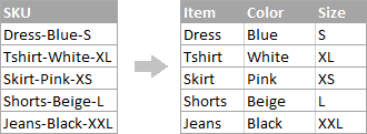
Supposing you have a list of SKUs of the Item-Color-Size pattern, and you want to split the column into 3 separate columns:
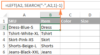
- To extract the item name (all characters before the 1st hyphen), insert the following formula in B2, and then copy it down the column:
=LEFT(A2, SEARCH("-",A2,1)-1)In this formula, SEARCH determines the position of the 1st hyphen ("-") in the string, and the LEFT function extracts all the characters left to it (you subtract 1 from the hyphen's position because you don't want to extract the hyphen itself).
- To extract the color (all characters between the 1st and 2nd hyphens), enter the following formula in C2, and then copy it down to other cells:
=MID(A2, SEARCH("-",A2) + 1, SEARCH("-",A2,SEARCH("-",A2)+1) - SEARCH("-",A2) - 1)
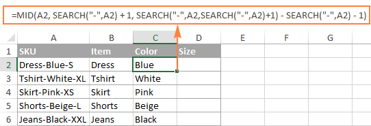
In this formula, we are using the Excel MID function to extract text from A2.
The starting position and the number of characters to be extracted are calculated with the help of 4 different SEARCH functions:
- Start number is the position of the first hyphen +1:
SEARCH("-",A2) + 1 - Number of characters to extract: the difference between the position of the 2nd hyphen and the 1st hyphen, minus 1:
SEARCH("-", A2, SEARCH("-",A2)+1) - SEARCH("-",A2) -1
- Start number is the position of the first hyphen +1:
- To extract the size (all characters after the 3rd hyphen), enter the following formula in D2:
=RIGHT(A2,LEN(A2) - SEARCH("-", A2, SEARCH("-", A2) + 1))In this formula, the LEN function returns the total length of the string, from which you subtract the position of the 2nd hyphen. The difference is the number of characters after the 2nd hyphen, and the RIGHT function extracts them.
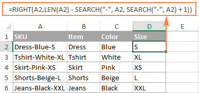
In a similar fashion, you can split column by any other character. All you have to do is to replace "-" with the required delimiter, for example space (" "), comma (","), slash ("/"), colon (";"), semicolon (";"), and so on.
Tip. In the above formulas, +1 and -1 correspond to the number of characters in the delimiter. In this example, it's a hyphen (1 character). If your delimiter consists of 2 characters, e.g. a comma and a space, then supply only the comma (",") to the SEARCH function, and use +2 and -2 instead of +1 and -1.
How to split string by line break in Excel
To split text by space, use formulas similar to the ones demonstrated in the previous example. The only difference is that you will need the CHAR function to supply the line break character since you cannot type it directly in the formula.
Supposing, the cells you want to split look similar to this:
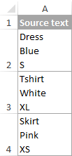
Take the formulas from the previous example and replace a hyphen ("-") with CHAR(10) where 10 is the ASCII code for Line feed.
- To extract the item name:
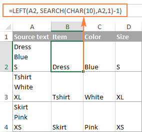
=LEFT(A2, SEARCH(CHAR(10),A2,1)-1) - To extract the color:
=MID(A2, SEARCH(CHAR(10),A2) + 1, SEARCH(CHAR(10),A2,SEARCH(CHAR(10),A2)+1) - SEARCH(CHAR(10),A2) - 1) - To extract the size:
=RIGHT(A2,LEN(A2) - SEARCH(CHAR(10), A2, SEARCH(CHAR(10), A2) + 1))
And this is how the result looks like:
How to split text and numbers in Excel
To begin with, there is no universal solution that would work for all alphanumeric strings. Which formula to use depends on the particular string pattern. Below you will find the formulas for the two common scenarios.
Split string of 'text + number' pattern
Supposing, you have a column of strings with text and numbers combined, where a number always follows text. You want to break the original strings so that the text and numbers appear in separate cells, like this:
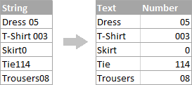
The result may be achieved in two different ways.
Method 1: Count digits and extract that many chars
The easiest way to split text string where number comes after text is this:
To extract numbers, you search the string for every possible number from 0 to 9, get the numbers total, and return that many characters from the end of the string.
With the original string in A2, the formula goes as follows:
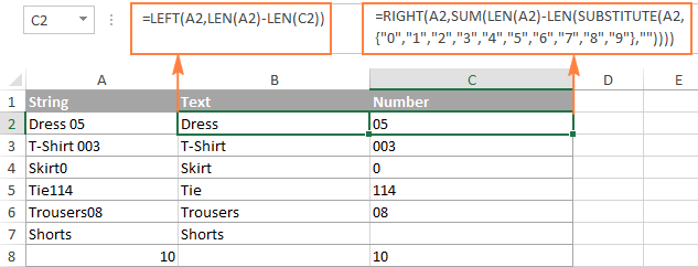
=RIGHT(A2,SUM(LEN(A2) - LEN(SUBSTITUTE(A2, {"0","1","2","3","4","5","6","7","8","9"},""))))
To extract text, you calculate how many text characters the string contains by subtracting the number of extracted digits (C2) from the total length of the original string in A2. After that, you use the LEFT function to return that many characters from the beginning of the string.
=LEFT(A2,LEN(A2)-LEN(C2))
Where A2 is the original string, and C2 is the extracted number, as shown in the screenshot:
Method 2: Find out the position of the 1st digit in a string
An alternative solution would be using the following formula to determine the position of the first digit in the string:
=MIN(SEARCH({0,1,2,3,4,5,6,7,8,9},A2&"0123456789"))
Once the position of the first digit is found, you can split text and numbers by using very simple LEFT and RIGHT formulas.
To extract text:
=LEFT(A2, B2-1)
To extract number:
=RIGHT(A2, LEN(A2)-B2+1)
Where A2 is the original string, and B2 is the position of the first number.
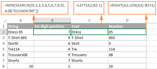
To get rid of the helper column holding the position of the first digit, you can embed the MIN formula into the LEFT and RIGHT functions:
Formula to extract text:
=LEFT(A2,MIN(SEARCH({0,1,2,3,4,5,6,7,8,9},A2&"0123456789"))-1)
Formula to extract numbers:
=RIGHT(A2,LEN(A2)-MIN(SEARCH({0,1,2,3,4,5,6,7,8,9},A2&"0123456789"))+1)
Split string of 'number + text' pattern
If you are splitting cells where text appears after number, you can extract numbers with the following formula:
=LEFT(A2, SUM(LEN(A2) - LEN(SUBSTITUTE(A2, {"0","1","2","3","4","5","6","7","8","9"}, ""))))
The formula is similar to the one discussed in the previous example, except that you use the LEFT function instead of RIGHT to get the number from the left side of the string.
Once you have the numbers, extract text by subtracting the number of digits from the total length of the original string:
=RIGHT(A2,LEN(A2)-LEN(B2))
Where A2 is the original string and B2 is the extracted number, as shown in the screenshot below:
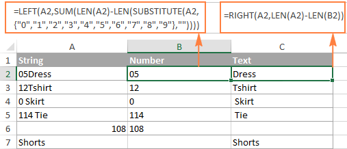
Tip. To get number from any position in a text string, use either this formula or the Extract tool. Or you can create a custom function to split numbers and text into separate columns.
This is how you can split strings in Excel using different combinations of different functions. As you see, the formulas are far from obvious, so you may want to download the sample Excel Split Cells workbook to examine them closer.
If figuring out the arcane twists of Excel formulas is not your favorite occupation, you may like the visual method to split cells in Excel, which is demonstrated in the next part of this tutorial.
How to split cells in Excel with Split Text tool
An alternative way to split a column in Excel is using the Split Text feature included with our Ultimate Suite for Excel, which provides the following options:
To make things clearer, let's have a closer look at each option, one at a time.
Split cells by character
Choose this option whenever you want to split the cell contents at each occurrence of the specified character.
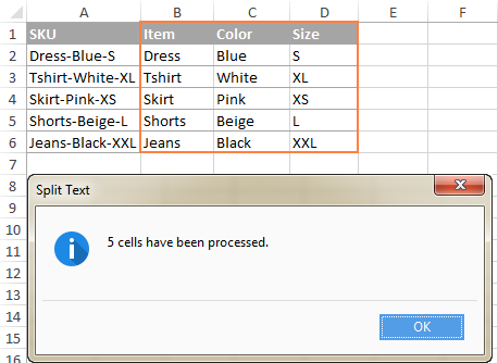
For this example, let's the take the strings of the Item-Color-Size pattern that we used in the first part of this tutorial. As you may remember, we separated them into 3 different columns using 3 different formulas. And here's how you can achieve the same result in 2 quick steps:
- Assuming you have Ultimate Suite installed, select the cells to split, and click the Split Text icon on the Ablebits Data tab.
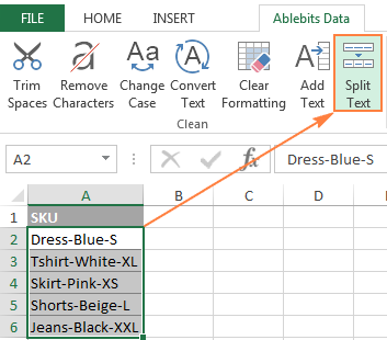
- The Split Text pane will open on the right side of your Excel window, and you do the following:
- Expand the Split by character group, and select one of the predefined delimiters or type any other character in the Custom box.
- Choose whether to split cells to columns or rows.
- Review the result under the Preview section, and click the Split button.
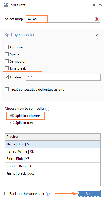
Tip. If there might be several successive delimiters in a cell (for example, more than one space character), select the Treat consecutive delimiters as one box.
Done! The task that required 3 formulas and 5 different functions now only takes a couple of seconds and a button click.
Split cells by string
This option lets you split strings using any combination of characters as a delimiter. Technically, you split a string into parts by using one or several different substrings as the boundaries of each part.
For example, to split a sentence by the conjunctions "and" and "or", expand the Split by strings group, and enter the delimiter strings, one per line:
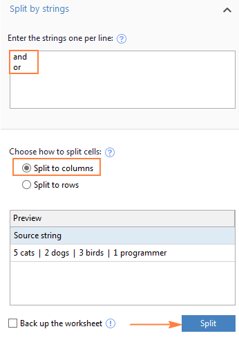
As the result, the source phrase is separated at each occurrence of each delimiter:

Tip. The characters "or" as well as "and" can often be part of words like "orange" or "Andalusia", so be sure to type a space before and after and and or to prevent splitting words.
And here another, real-life example. Supposing you've imported a column of dates from an external source, which look as follows:
5.1.2016 12:20
5.2.2016 14:50
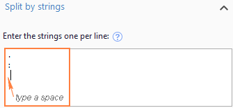
This format is not conventional for Excel, and therefore none of the Date functions would recognize any of the date or time elements. To split day, month, year, hours and minutes into separate cells, enter the following characters in the Split by strings box:
- Dot (.) to separate day, month, and year
- Colon (:) to separate hours and minutes
- Space to separate date and time
Hit the Split button, and you will immediately get the result:

Split cells by mask (pattern)
Separating a cell by mask means splitting a string based on a pattern.
This option comes in very handy when you need to split a list of homogeneous strings into some elements, or substrings. The complication is that the source text cannot be split at each occurrence of a given delimiter, only at some specific occurrence(s). The following example will make things easier to understand.
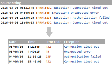
Supposing you have a list of strings extracted from some log file:

What you want is to have date and time, if any, error code and exception details in 3 separate columns. You cannot utilize a space as the delimiter because there are spaces between date and time, which should appear in one column, and there are spaces within the exception text, which should also appear in one column.
The solution is splitting a string by the following mask: *ERROR:*Exception:*
Where the asterisk (*) represents any number of characters.
The colons (:) are included in the delimiters because we don't want them to appear in the resulting cells.
And now, expand the Split by mask section on the Split Text pane, type the mask in the Enter delimiters box, and click Split:
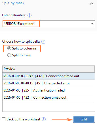
The result will look similar to this:

Note. Splitting string by mask is case-sensitive. So, be sure to type the characters in the mask exactly as they appear in the source strings.
A big advantage of this method is flexibility. For example, if all of the original strings have date and time values, and you want them to appear in different columns, use this mask:
* *ERROR:*Exception:*
Translated into plain English, the mask instructs the add-in to divide the original strings into 4 parts:
- All characters before the 1st space found within the string (date)
- Characters between the 1st space and the word ERROR: (time)
- Text between ERROR: and Exception: (error code)
- Everything that comes after Exception: (exception text)
I hope you liked this quick and straightforward way to split strings in Excel. If you are curious to give it a try, an evaluation version is available for download below. I thank you for reading and hope to see you on our blog next week!
Available downloads
Excel Split Cells formulas (.xlsx file)
Ultimate Suite 14-day fully-functional version (.exe file)
 by
by
306 comments
Hello, I have a long text in one column and I need to split it into different sections. When I tried to split by all "," "." " " I have over 5000 columns. Anyone who might help ?
Part of the text in one column:
Zsolt Geretovszky University of Szeged, Hungary,2,33,16.50.Ziming Zhong 1,56,56.00,Giorgio Maddaluno.Zhixian X Jiu Wuhan Polytechnic University, China,2,4,2.00.
Wanted result: (bigger spaces = different columns - f.e. Zsolt Geretovszky is name, university of szeged is school etc.)
Zsolt Geretovszky University of Szeged Hungary 2 33 16.50
Ziming Zhong 1 56 56.00
Giorgio Maddaluno
Zhixian X Jiu Wuhan Polytechnic University China 2 4 2.00
Hello!
Your data doesn't have a pattern. Space is used in the first and last name, and between the first name and the school. The period is used in numbers and to separate records. I cannot help you.
my data in one column:
GLES2_IMPL_EXPORT extern const char kEnableGpuClientTracing[]
GPU_EXPORT extern const char kDisableShaderNameHashing[]
extern const char kNearbyShareHTTPHost[]
COMPONENT_EXPORT(ASH_CONSTANTS) extern const char kArcDisableAppSync[]
And i need:- kEnableGpuClientTracing[]
kDisableShaderNameHashing[]
kNearbyShareHTTPHost[]
kArcDisableAppSync[] to be seperated.
When I'm using the formulae it got separated with "extern const char kDisable....."
could you help me through this?
Hi!
Your question is not clear. Do you want to get the last word in the text? Explain in more detail.
I have a comma delimited list of zip codes that I need split into 1200 character max lengths while still keeping the zip codes together, but not going over 1200 characters. Is there any formula that will do that so I don't have to manually do it?
Thanks!
Just to clarify - they are all in one cell and it is 8747 characters in one cell. I'd like to have cells that are no more than 1200 characters in length, without breaking apart the zip codes. Thanks!
Hello!
Such long text can be split into cells only with a special tool. I recommend paying attention to the Split Text Tool.
Hi,
I would like to split an 11 digits sequence e.g. 23456543987 into 11 separate cells in excel.
Can you please advise me?
thanks a lot.
Hello!
You can use the formula:
=MID($A$1,ROW(A1),1)
After that, you can copy this formula down along the column.
thank you Alexander
Go to Data > Text to Columns and set delimiter to -
Hi,
In cells of Column A I have data:
55771 13 units
44231 5 units
12341 22 units
and etc....
In adjacent cells of Column B I need:
55771
44231
12341
In adjacent cells of Column C:
13 units
5 units
22 units
Is it possible with formula?
Hello!
The formula below will do the trick for you:
=LEFT(A1,SEARCH(" ",A1,1)-1)
and
=MID(A1,SEARCH(" ",A1,1)+1,50)
Is there any chance to do it with one formula?
Hello!
The formula changes the value only in the cell in which it is written. You have 2 columns, so you need 2 formulas. Or write a VBA macro.
Ok, Thank you
Hi, please help me out.
Column A has,
7000
12345
54543
7890
it has to be separated into two units from the last and to be written in columns B, C and D... like...
In Column B
00
45
43
90
In column C
70
23
45
78
In column D
0
1
5
0
(zero- since there are no more digits there)
Please help me with the formula.
Thanks.
Hello!
Use formulas
=MID(A2,LEN(A2)-1,2)
=MID(A2,LEN(A2)-3,2)
=IFERROR(MID(A2,LEN(A2)-4,1),0)
You can learn more about MID function in Excel in this article on our blog.
Cell has string of 6 digit numbers: A1=123456 234567 345678 456789 ... Split the string of 6-digit numbers into single column, B1=123456, B2=234567, B3=345678, B4=456789, .... Any suggested solution? Thank you.
Hello!
You can use the Split Text tool as described in the article above. Then you can write the obtained results into a column using the Transpose Range tool.
It is available as a part of our Ultimate Suite for Excel that you can install in a trial mode and check how it works for free.
Try using:
=MID($A$1,IF(ROW(A1)>1,(ROW(A1)-1)*6+1,ROW(A1)),6)
This will read the row the formula is on and give you the 6 characters from that row's set
Drag the formula down for as many rows as there are data sets in cell A1
Hi, My query is that if we have first names and last names combined in a column (with both of them starting with capital letters) then is it possible to separate the strings into first name and last name? both the first and last names have different number of characters.
Hello!
I recommend reading this guide: How to separate names in Excel- split first and last name into different columns.
Hope you’ll find this information helpful.
Thank You!!
012-01-I-020-RUBBER RUNNER SET
I WANT TO SPLIT ABOVE DATA AS BELOW
012-01-I-020 IN ONE CELL AND RUBBER RUNNER SET IN ANOTHER CELL
my data actual data as below which i want to split.
012-01-I-020-RUBBER RUNNER SET
01-U-428-UNWINDER UN SCREW AND FLANGE ASSY M104
02-P-458-FR 59-48 1080 28 1334 MS/MS 104
03-C-096-CUTTING BRIDGE ASM FOR Ø130ROTARY(M-104)
03-C-4016-GFR 44-32 360 25 386 MS/MS 104
09-01-S-142-TOP & BOTTOM KNIFE BRKT-L.H 60MM WIDTH
Hi!
The answer to your question is in the first paragraph of this article.
I'm looking to split Name, address, city, state, zip in their own columns. As of now, they are in 1 column
Name Address City, State Zip
Thank you for any help!!
HI, id really love your help on this
I'm trying to split the below into columns, I'm doing ok with the =LEFT formula but trying to split the rest is proving difficult
WIFI:T:WPA;S:RUT240_93AD;P:k2T6Vvu5;;SN:1107473141;I:861585044986089;M:001E422B93AB;B:081;
For example, anything after the ":" is what im trying to get.
Eg - values ONLY after S: RUT240_93AD, P: k2t6Vvu5, SN: 1107473141
I would like just the model and serial numbers in their own column, without the "S:" attached to it
Hello!
If I got you right, the formula below will help you with your task:
=MID(A1,SEARCH("S:",A1,1)+2,SEARCH("I:",A1,SEARCH("S:",A1,1))-3-SEARCH("S:",A1,1))
I hope my advice will help you solve your task.
Hi,
I have a scenario where I get string followed by numbers as below in a cell. Sometimes it won't be in sequential order. I am able to split it taking ";" as delimiter. But not able to sort and find min value, max value as it is a string followed by number.
Integration Sprint 34;Integration Sprint 35;Integration Sprint 36;Integration Sprint 37;Integration Sprint 38;Integration Sprint 39;Integration Sprint 40
I need to split it considering ";" as delimiter and sort it in sequential order.
Then i need to find minimum value and max value
Could you please suggest excel tips for it
Hi!
We have tools that can solve your task in a couple of clicks - Split Tool and Extract tool. You can split text into rows with semicolon delimiters, and then extract numbers from each cell.
It is available as a part of our Ultimate Suite for Excel that you can install in a trial mode and check how it works for free.
I hope I answered your question. If something is still unclear, please feel free to ask.
Hello,
I have this table
ID(size-no.of purchase)
2-1
2-1
2-4
1-1,2-1,13-1
2-1
2-1
10-1
1-1
2-1
2-1
3-1
3-1
2-1
3-1
3-2
5-1,10-1,1-1,6-1
3-1
3-1
3-1
3-1
2-1,1-1,3-1
3-1
3-1
3-1
2-1,1-1
1-1
3-1
5-1
5-1
5-1
5-1
2-1
2-1
2-1
1-1
5-1
2-1
1-1
2-1
5-1
5-1
1-1,3-2,2-1,13-1
2-1,1-1,3-1
2-1,1-1,3-1
3-1
1-1,3-1,2-1
5-1
5-1,10-1
2-1,1-1
2-1,1-1
5-2
1-1
3-1
5-2
1-2,2-2
1-1
3-1
10-1,1-1
1-1,3-1,2-1
1-1,3-1,2-1,13-1
1-1,2-1,3-1
5-1,10-1,1-1,6-1,3-1,9-1
5-1
how to split and find sum of purchase?
Thanks for Response!
Hi!
Explain what this data means and by what numbers you want to find the amount.
Please I want to separate N1,N2,N3 up to N48 in a cell to 48 cells
Hello!
Use the Split Text feature as described above. It is available as a part of our Ultimate Suite for Excel that you can install in a trial mode and check how it works for free.
Hey there.
I have a text like this in one cell:
"ABC: fdsdfsfdsdfds.ghfhghjhf.BCD: ghgfhfhhgfg.CDE: tretrerter.DEF: hgfhgfhggf."
where those labels (ABC, BCD, CDE, DEF) can be a single or multiple words and they are always followed by ':'.
What I'd like to get is
1) to split those blocks in different columns
2) to get the label for each of these new columns.
So it would be something like:
label1: "ABC"
text1: "fdsdfsfdsdfds.ghfhghjhf." (it's ok also to get "ABC: fdsdfsfdsdfds.ghfhghjhf.")
label2: "BCD"
text2: "ghgfhfhhgfg." (it's ok also to get "BCD: ghgfhfhhgfg.")
label3: "CDE"
text3: "tretrerter." (it's fine ok to get "CDE: tretrerter.")
label4: "DEF"
text4: "hgfhgfhggf." (it's ok also to get "DEF: hgfhgfhggf.")
I'm having problems detecting the delimiter for splitting, given that it can't be always (as you can see ABC should result = fdsdfsfdsdfds.ghfhghjhf.). So delimiter should be but only when it's followed by ':' prior to ...
Any idea about how I can do it?
Thanks.
Hi!
The separator, in your case, is the text between period and colon. But in your data, the period is both a separator and a regular character at the same time. I don't think I can help you.
For the string 100005.5559Dress, (IN CELL A2)
using the = LEFT(A2,SUM(LEN(A2)-LEN(SUBSTITUTE(A2,{"0","1","2","3","4","5","6","7","8","9"},"")))),
output is as followed:
100005.555
NOT 100005.5559.
Please advise an amended code to have 100005.5559 reflected as the output.
Hello!
You need to add one more symbol to your formula: "."
=LEFT(A2,SUM(LEN(A2)-LEN(SUBSTITUTE(A2,{"0","1","2","3","4","5","6","7","8","9","."},""))))
This should solve your task.
Hi Folks,
This helped me with some of my task, but there is one section I can't seem to extract. I have a string from a barcode scanner that looks like this:
B55032324d12200420222537\r\n31483\r\n086-118090-900\r\nNWK12200420222536
And I want to break it apart at the "\r\n" in separate cells, the order or orientation is not important.
Hello!
Writing a formula to separate 4 words is a very difficult task. I recommend split text with the Split Text feature.
It is available as a part of our Ultimate Suite for Excel that you can install in a trial mode and check how it works for free.
Thanks !!! you saved my life <3
Super useful. I used it to separate out the domain in email addresses so I could see which emails were in the same domain like this....
=LEFT(B2, SEARCH("@",B2,1)-1)
=RIGHT(B2,LEN(B2)- SEARCH("@",B2,1))
tabel Size w h A W H B&c W H D Or D&E
Freezer : A - W: 48” x H: 28” | B & C - W: 26” x H: 30”|D - W: 48” x H: 26” 48 28 1 26 30 2 48 26 1
Freezer : A - W: 64” x H: 29” | B & C - W: 27.5” x H: 21”D & E - W: 28” x H: 39” 64 29 1 27.5 21 2 28 39 2
Freezer : A - W: 61” x H: 25” | B & C - W: 23” x H: 21”D & E - W: 25” x H: 29” 61 25 1 23 21 2 25 29 2
Thank you!!!
I have applied the following formula to my spreadsheet to split 1 cell that contains the information as follows:
Cell = 3^4^12
With the formula applied, the cell is split and separated into their own separate cells as follows:
3
4
1
The issue is that the formula I've applied does not taken into account that there may be numbers of more than 1 digit.
So instead of the intended outcome being:
3, 4, 12, the formula splits it as 3, 4 and 1
Please advise if there is a way to solve this issue?
formula to split 1st number:
=LEFT(D3,SEARCH("^",D3)-1)
formula to split 2nd number:
=IFERROR(MID(D3,SEARCH("^",D3)+1,SEARCH("",D3,SEARCH("^",D3)+1)-SEARCH("^",D3))," ")
formula to split 3rd number:
=IFERROR(MID(D3,SEARCH("^",D3)+3,SEARCH("",D3,SEARCH("^",D3)+1)-SEARCH("^",D3))," ")
Hello!
To split the text into 3 parts, you can use this tutorial: How to split full name to first, last, and middle name.
If this task needs to be solved often, I'd recommend you to have a look at our Split Names tool.
I hope it’ll be helpful.
INPUT DATA
Column A
(Blank)
(Blank)
ABCDEFGHI
JKLMNO
PQRS
UVWX
NEED OUTPUT
COLUMN B
ABCDEFGHI
COLUMN c
JKLMNO
COLUMN D
PQRS
COLUMN e
UVWX
Hi!
If I understand your task correctly, the following tutorial should help: How to convert rows to columns in Excel (transpose data).
Hi. I have the below data, each containing information separated by the "^" sign.
The length of this data is not consistent, with some containing 2 "^" and others with up to 15 "^"
I've tried the LEFT, MID, RIGHT formula, but I do not know how to extend it to search up to 15 "^"
Please can you help.
Data:
Colour (heading)
Orange^Black^Red^Yellow^Grey
Colour Reference (heading)
O^BL^R^Y^GY
Colour QTY to Order (heading)
1000^1500^1300^500^2000
I would like to split the data in each row, into it's own column/row
So that in the end:
Colour QTY to Order
1000 - each in it's own row/column
1500
1300
500
2000
Hello!
To split text into cells, you can use Split Text feature. It is available as a part of our Ultimate Suite for Excel that you can install in a trial mode and check how it works for free.
You can use the Text to Columns tool. Read more about it in this article.
I hope it’ll be helpful.
Thank you for the quick reply.
I was hoping there was a formula I could use, so that when the s/sheet is auto-populated with data, I can then add a formula that will automatically split the columns, as opposed to using Text to Columns.
Please let me know.
Thanks
Joanne
Hi Joanne,
Assuming the titles of the columns are the values you are searching for you can get your table with a single formula.
Titles like O, BL, R, Y, GY in B1:Z1
Data into A2
O^BL^R^Y^GY
B^GR^1000
B^GR^Y
RD^5000
1000^5000 etc
Into B2 put the following :
=IFERROR(IF(FIND("^"&B$1&"^","^"&$A2&"^")>0,B$1,""),"")
drag formula to cover span of the table.
I've added manually ^ to each end of the string to search to ensure all values are found (in case one end is missing a character)
If it finds the ^xx^ in the string it puts it in the matching titles column.
After using Python for years, it almost seems criminal that Excel doesn't include a "split" command within the UI. I created my own user-defined function (UDF) to accomplish this. This parser can pluck the Nth element from a given string provided there's a consistent delimiter, and it can work left to right or right to left. Code:
Option Explicit
Function GetLength(a As Variant) As Integer
If IsEmpty(a) Then
GetLength = 0
Else
GetLength = UBound(a) - LBound(a) + 1
End If
End Function
Function FetchElement(RefCell As String, ReturnElementNbr As Integer, Delimiter As String, Reverse As Boolean) As String
Dim Hierarchy As String
Dim MyArray As Variant
Dim ArraySize As Integer
If Reverse = True Then
If Right(RefCell, 1) = Delimiter Then
Hierarchy = StrReverse(Left(RefCell, Len(RefCell) - 1)) 'remove trailing "\" and then reverse remainder of string
Else: Hierarchy = StrReverse(RefCell)
End If
Else: Hierarchy = RefCell
End If
MyArray = Split(Hierarchy, Delimiter)
ArraySize = GetLength(MyArray)
If ReturnElementNbr > ArraySize Then
FetchElement = ""
ElseIf Reverse = True Then FetchElement = StrReverse(MyArray(ReturnElementNbr - 1))
Else: FetchElement = MyArray(ReturnElementNbr - 1)
End If
End Function
sample data to parse (let's say it's in cell "A1"): prvd00664966\PT00076084\PT00072170\PT00072157\PT00076116
command: =FetchElement(A1,3, "\", TRUE)
this will count the elements from right to left (TRUE flag used) with an assumption that the delimiter is a "\" and that we want the third element (parm = 3, above) in the list.
Yes, UDFs are relatively slow. But this is a heck of a lot more readable and usable than having to use so many nested string functions in Excel
Thank you for your instructions. Unfortunately I could not find my answer. If you could be so kind to help me. I have the following data:
For example (123)
For example (1)
For (example) (344)
For example (for) example (12)
I need to remove the numbers and the brackets. I tried many ways but I have not found a solution. There is a formula for removing everything after and including brackets. However then I have a problem with data such as: For example (for) example (12) . In which it will not only delete the numbers but also the text.
Is there a formula for deleting numbers in brackets? Or a way for me to remove it?
Hope to hear from you soon.
Hello!
Here is the formula that should work perfectly for you:
=SUBSTITUTE(SUBSTITUTE((CONCAT(IF(NOT(ISNUMBER( --MID(A1,ROW($1:$93),1))), MID(A1,ROW($1:$93),1),"")))," ",""),"()","",1)
We have a tool that can solve your task in a couple of clicks — Ablebits Data - Remove Characters. It is available as a part of our Ultimate Suite for Excel that you can install in a trial mode and check how it works for free.
Hi There,
How do I separate text by a pattern. However, the pattern can change and there is no common string that I can use to separate the cell into columns.
For example,
I have the text 2015 Mazda CX5 V6 White Bumper. I would like to split this by Make, Model, Year, Engine Type, Color, Part and others if any. The tricky part here is on the next row I could have 2003 Toyota Camry Bonnet Blue. I want all the makes to go into 1 column, all the models to go into 1 column, all the parts to go into 1 column and so on. The pattern can change as well. Because sometimes it can start with the make and end with model or it could be other as well. I want this process to be automated.
Because the excel wouldn't understand what the make, model, year are, what we could do is we could probably add a drop-down on the heading of each column that has the list of makes, and another column would be models and so on. So, now when the system identifies make, it would have to search in all the drop-downs of all the columns and find where it is and put it on that column. I know it's a little complex, but I am sure it can be done.
Any help would highly be appreciated. Thank you!!
The goal is to split each Biblical Hebrew word into individual letters. However, Text-to-Column causes the nikkud/accents to separate from the base letter.
I've discovered that putting a hyphen between each letter of the Hebrew word will cause Text-to-Column to separate the individuals characters intact.
So, I went looking for a formula to insert dashes between letters and found one that works....but only for English letters/numbers. With the Hebrew, this formula separates out the nikkud/accents.
https://superuser.com/questions/1371473/how-can-i-format-a-character-string-in-excel-to-insert-hyphens
Sub InsertCharacter()
Dim Rng As Range
Dim InputRng As Range, OutRng As Range
Dim xRow As Integer
Dim xChar As String
Dim index As Integer
Dim arr As Variant
Dim xValue As String
Dim outValue As String
Dim xNum As Integer
xTitleId = "Put Dashes"
Set InputRng = Application.Selection
Set InputRng = Application.InputBox("Range :", xTitleId, InputRng.Address, Type:=8)
xRow = Application.InputBox("Number of characters :", xTitleId, Type:=1)
xChar = Application.InputBox("Specify a character :", xTitleId, Type:=2)
Set OutRng = Application.InputBox("Out put to (single cell):", xTitleId, Type:=8)
Set OutRng = OutRng.Range("A1")
xNum = 1
For Each Rng In InputRng
xValue = Rng.Value
outValue = ""
For index = 1 To VBA.Len(xValue)
If index Mod xRow = 0 And index VBA.Len(xValue) Then
outValue = outValue + VBA.Mid(xValue, index, 1) + xChar
Else
outValue = outValue + VBA.Mid(xValue, index, 1)
End If
Next
OutRng.Cells(xNum, 1).Value = outValue
xNum = xNum + 1
Next
End Sub
Question: Is there a way to tweak this formula so that it will recognize Hebrew 'complete characters'? Or is there another way to work with Hebrew in Excel?
Thanks so much.
problem string:
/subscriptions/dummy-subscription-id/resourceGroups/my-resource-group-name/providers/Microsoft.Web/serverfarms/my-app-service-plan-name
what i needed out of it?
my-app-service-plan-name
what expression got it?
=RIGHT(I2,LEN(I2)-SEARCH("serverfarms",I2)-LEN("serverfarms"))
thanks for guiding me towards
Super thanks to you, you made my day really grate
whith this formular :
=LEFT(A10,LEN(A10)-LEN(D10))
I need to split the value 12 into 9 2 1 in 3 different cellsand incase if the value becomes 13 i need it to ne splited inti 9 2 2. Is that possible? I need the value in the last colum keep changing if the value varies. Is there any possibile solution? Please help
Hello!
If I understand your task correctly, the following formula should work for you:
=D1-9-2
Hope this is what you need.
Looking for an automatic option to take whatever is typed into cell B3 to auto populate each character into rows beneith
Ex: B3 =abcd 'is entered
cells populate here:
Cells B5 =a
B6 = b
B7 = c
B8 = d
cannot use text to column
Any help???
Use the MID function. Write down the formula in B5
=MID($B$3,ROW()-4,1)
Copy this formula down column B.
I hope it’ll be helpful.
HI,
I am looking for the number "02305255" to be separated from the hyperlink. Could you help get the Excel formula?
Hello!
Please check out the following article on our blog, it’ll be sure to help you with your task: Excel Hyperlink: how to create, change and remove
I hope this will help, otherwise please do not hesitate to contact me anytime.
Thank you for the helpful article and comments!
I have been trying to separate a string into characters (so I can have each character into a separate column).
Such as if I have a string “word”, I would like to to have it’s characters “w”, “o”, “r”, “d” in separate columns.
Any help will be appreciated.
Hello!
If your text is written in cell A1, write the formula in B1:
=MID($A$1,COLUMN()-1,1)
Copy this formula column by column to C1, D1, E1, etc.
I hope it’ll be helpful.
Thanks!
Thank you!
I am using AbleBits Split by Characters function to split by commas into rows. No matter how many times I try it, it splits into columns instead. Can you help me understand what I'm doing wrong?
Hello!
Unfortunately, without seeing your data it is impossible to give you advice.
I'm sorry, it is not very clear what result you want to get. Could you please describe your task in more detail and send us a small sample workbook with the source data and expected result to support@ablebits.com? Please shorten your tables to 10-20 rows/columns and include the link to your blog comment.
We'll look into your task and try to help.
I cannot get a cell separated and have it still identified as a whole number (to later average). I’ve tried substitute, replace, left functions... with no luck.
It is separating out the _F from a number of temperature readings: 37 F, 42 F, etc
Lil help?
Hello!
To remove characters and convert to a number, use the formula
=--SUBSTITUTE(E1," F","")
I hope it’ll be helpful.
Hi,there!
I want to separate # following with any number for example #8, #6, then I want to use number 8 or 6 as my value to use if function to print out different result, if 8 , print " 38 mm", if 6 print " 50mm" just a example. Thanks a lot!
"I want to separate # following with any number for example #8, #6, then I want to use number 8 or 6 as my value to use if function to print out different result, if 8 , print " 38 mm", if 6 print " 50mm" just a example. Thanks a lot!" It is in the Same Cell, print also at the same Cell.
Hello!
I’m sorry but I do not fully understand your goal. If you want to replace the entered value 8 with the text in the same cell, then this is possible only using a VBA macro. You can write either a value or a formula in a cell. If you need to convert # 8 to a number, you can use the formula
=--SUBSTITUTE(A2,"#","",1)
or
=IF(SUBSTITUTE(A2,"#","",1)="8","38mm",IF(SUBSTITUTE(A2,"#","",1)="6","50mm",""))
I have a cell like "1 S Laser Beam, 3 M Pulse Laser, 18 Sansha Debris, 9 M Booster"
what this means is that the cell has 1 qty of Small Laser Beam, 3 qty of Medium Pulse Lasers and etc.
How can I parse this so that I can parse these quantities so that I can use them individually? Thanks
Hello!
You can split your text into cells in any of the ways described above. Use a comma as a separator. You can then extract a number from each cell using a formula. For example:
=--LEFT(A1,FIND(" ",A1,1)-1)
I hope it’ll be helpful.
Hi there,
How to split this? Can you tell me?
151 Exc AvenueNey York, NY 10001
123 Word AptMiami, FL 23456
I Want city name to be in separate field and presiding address in separate field. Any formula which puts the word starting in CAPITAL after SMALL letter to a different field?
I have a challenge on number search in a cell that is formatted as text. I have a TAB "Systems Software" with column G that have cells with multiple numbers (not necessarily in numeric order) separated by commas (i.e., G4 contains 4,28,9,14,44,23,10,104) in each cell. Each cell may have a single number, or be empty or a string of numbers separate by a commas. I need to find if a given specific number (i.e., 4) is in that string of numbers that are contained in a cell formatted as text. It is number four that I am searching for in that sample, not the four in fourteen or forty four or one hundred four. If I find the search number within the number in the string, I can print an X in the cell that is doing the search. Otherwise, if the number is not found, leave the cell empty. Any help will be greatly appreciated.
Looking for just 4 and not the 4 in 14,24,104 etc?
Simply search for ",4," Include the commas.
The only time you need any special check is the first or last numbers in the string.
Saiph
Hi Team,
He is a smart guy.
smart people are everywhere.
I want to print the word which is right after the word "smart", can some one please help me
Thanks,
Anand
Hello!
If I understand your task correctly, the following formula should work for you:
=MID(B1,SEARCH("smart",B1,1)+6,LEN(B1)-(SEARCH("smart",B1,1)+5))
I hope this will help
For those wondering how to split a chain of characters into more than 3 cells :
I'm too lazy to translate my formulas. The functions are in french so I'll just translate them here :
GAUCHE = LEFT
DROITE= RIGHT
STXT= MID
CHERCHE= SEARCH
NBCAR= LEN
So, I wrote in A2 (yeah I started from A2 instead of A1) :
test1;test2;test3;test4;test5;test6
I want to separate this into 6 cells.
In B2, I type :
=GAUCHE(A2;(CHERCHE(";";A2;1)-1))
This gives me "test1".
In C2, I type :
=STXT(A2;NBCAR(B2)+2;CHERCHE(";";A2;(NBCAR(B2)+2)-CHERCHE(";";A2))-1)
This gives me "test2"
In D2, I'll write :
=DROITE(A2;NBCAR(A2)-NBCAR(B2)-NBCAR(C2)-2)
This gives me "test3;test4;test5;test6"
From there on, I can reiterate the two other formulas to obtain in E2 : "test3", in F2 : "test4", in G2 : "test5;test6" and so on and so on.
Hi Team - Thanks for this material.. absolutely useful. However I am a bit stuck (think i am being naive as missing something :) ).. From example above, how am i able to split all the string between 2 characters as there are multiple occurrences.
Above example shows clearly on how to extract between 1st and 2nd occurrence. How about 2nd and 3rd occurrence, 3rd and 4th occurrence etc.. I want this to be in a single formula.
Example:
Dress-Blue-S-US-20-Yes
Expected output:
Blue (Answer available on top of this post)
S
US
20
Yes
Hello!
Dividing a long text into separate words using a formula is a very difficult task. If the text contains more than 4 words, then solving the problem using the formula does not make sense. Use the standard Text to Columns tool or the Ablebits Split Text tool, which is described earlier in this article.
Hi - Unfortunately i cannot use the options in Excel as I can only use it via formula due to the fact that the incoming value string is a variable that will be written at runtime & has to be decoded into above requirement during playback/runtime
Thanks
=TextSplit(TextAfter([SourceCell], "-"), , "-") will parse everything after the first "-" into separate cells in a row below the cell containing this formula, just as you have in your example.
I am working with power query and my results have jumbled together movie names with release dates, where the release date (format August 7, 2020) is combined with the movie name. the movie names of course are different lengths, and the dates are different lengths depending on the release date. I'm not finding any way to split my data between the movie name and the release date (example: The Broken Hearts GalleryAugust 7, 2020). Can you show me how to do this?
Hello Michael!
To separate the date from the text, you can use the formula
=RIGHT(F1,LEN(F1)-FIND("~",SUBSTITUTE(F1," ","~",LEN(F1)-LEN(SUBSTITUTE(F1," ",""))-2)))
I hope my advice will help you solve your task.
I’ve found one way that adds a small macro (that you don’t need to keep)
ALT + F11
Create a module and add the following code:
Function IS_DATE(rng) As Boolean
IS_DATE = IsDate(rng)
End Function
This will tell you if a date is valid or not (true/false)
Then we test your movie titles by trying to find the date on the end
There will always be 4 digits for year, 1 for comma, 1 space, at least one digit for day and then the month. A span of 7 possible lengths. May x – September xx
Assuming your title/date is in A1.
In B1 put:
=IF(is_date(RIGHT(A1,11))=TRUE,11,IF(is_date(RIGHT(A1,12))=TRUE,12,IF(is_date(RIGHT(A1,13))=TRUE,13,IF(is_date(RIGHT(A1,14))=TRUE,14,IF(is_date(RIGHT(A1,15))=TRUE,15,IF(is_date(RIGHT(A1,16))=TRUE,16,IF(is_date(RIGHT(A1,17))=TRUE,17,IF(is_date(RIGHT(A1,18))=TRUE,18,""))))))))
The formula trys cropping the string at 11 characters long to 18 and tests each one to see if it’s a real date or not. The month is the decider so short spelled or additional characters make this a false date. Only the right length will actually create a valid date and returns the trim length
The result is the number of characters to cut the string at
Movie title goes in C1:
=left(A1,len(A1)-B1)
Date goes into D1
=right(A1,B1)
Hi..
Plz help me to count the frequency in the following
1234567 = frequency is 7 than plz help me to find correct formula for count frequency in the following examples
1.3..67 = 4 and
7 = 1 and
...3...7 = 2
Plz help
Hello!
Tell me specifically what exactly you want to calculate. "1234567 = frequency is 7" is not a frequency. Perhaps you want to find the number of digits? Or the number of characters? Or something else?
Hello,
I'am looking for this function:
I have a cell like this : XTORM SOLID BLUE MICRO USB CABLE 1MTR
I want to split this cell (all cells with text) after the 3rd or 4rd space, like this
XTORM SOLID BLUE
MICRO USB CABLE
1MTR
Those words undernead in 1 cell
Is this possible?? i hope thanks!!! greetz remco
Hello Remco!
To divide the text into 3 cells after every third space, use the formulas
=LEFT(C1,FIND("*",SUBSTITUTE(C1," ","*",3))-1)
=MID(C1,FIND("*",SUBSTITUTE(C1," ","*",3))+1, FIND("*",SUBSTITUTE(C1," ","*",6)) -FIND("*",SUBSTITUTE(C1," ","*",3)))
=IFERROR(MID(C1,FIND("*",SUBSTITUTE(C1," ","*",6))+1, FIND("*",SUBSTITUTE(C1," ","*",9))-FIND("*",SUBSTITUTE(C1," ","*",6))), MID(C1,FIND("*",SUBSTITUTE(C1," ","*",6))+1, LEN(C1)-FIND("*",SUBSTITUTE(C1," ","*",6))))
I hope this will help
Thank you!
I have output from a Qualtrics survey for "select all that apply" questions. I need to import it into a statistical package for analysis (SPSS). The data now have numeric codes for answer choices, but when imported into the stats package are read as string (alpha) and separated by commas. I am trying to use Exsel to separate these values into columns, but need a different column for each value. Some questions have up to 5 values, but users may have only checked 1, 2 or even 4 or 5 options, and so their values vary.
Original Data: --> New array, where | | indicates a separate column
1, 2, 5 becomes | 1 | 2 | | | 5| (i.e. the columns for the values 3 and 4 are left blank)
2, 3, becomes | | 2 | 3 | | | (i.e. the columns for the values 1, 4 and 5 are left blank)
4 becomes | | | | 4 | | (i.e. the columns for the values, 1, 2, 3 and 5 are left blank)
Text to column separates them, but then I have a column with a mixture of answers (e.g. 1, 2, 4 based on example above) yet I need to create a dichotomous variable for answer choice 1, a separate one for 2, etc. Any ideas? Thank you.
I don't know if you can do it other than with a formula:
______A___ | ____________B______________ ... ____________F______________
1 | "1,2,5" | =if(iserr(find("1",A1)),"",1) ... =if(iserr(find("5",A1)),"",5)
2 | ...
3 | "4" ____| =if(iserr(find("1",A3)),"",1) ... =if(iserr(find("5",A3)),"",5)
Hello Sara!
If I understand your task correctly, please try the following formula:
For example, the value of cell A1 is 1,2,5
Formula in cell B1
=IFERROR(IF(--FIND("1",A1,1) > 0,1,""),"")
Formula in cell C1
=IFERROR(IF(--FIND("2",A1,1) > 0,2,""),"")
Formula in cell D1
=IFERROR(IF(--FIND("3",A1,1) > 0,3,""),"")
Formula in cell E1
=IFERROR(IF(--FIND("4",A1,1) > 0,4,""),"")
Formula in cell F1
=IFERROR(IF(--FIND("5",A1,1) > 0,5,""),"")
I hope this will help, otherwise please do not hesitate to contact me anytime.