The tutorial explains how to use the nested IF function in Excel to check multiple conditions. You will also learn a few other functions that could be good alternatives to using a nested formula in Excel.
How do you usually implement a decision-making logic in your Excel worksheets? In most cases, you'd use an IF formula to test your condition and return one value if the condition is met, another value if the condition is not met. To evaluate more than one condition and return different values depending on the results, you nest multiple IFs inside each other.
Though very popular, the nested IF statement is not the only way to check multiple conditions in Excel. In this tutorial, you will find a handful of alternatives that are definitely worth exploring.
Excel nested IF statement
Here's the classic Excel nested IF formula in a generic form:
You can see that each subsequent IF function is embedded into the value_if_false argument of the previous function. Each IF function is enclosed in its own set of parentheses, but all the closing parentheses are at the end of the formula.
Our generic nested IF formula evaluates 3 conditions, and returns 4 different results (result 4 is returned if none of the conditions is TRUE). Translated into a human language, this nested IF statement tells Excel to do the following:
test condition2, if TRUE - return result2, if FALSE -
test condition3, if TRUE - return result3, if FALSE -
return result4
As an example, let's find out commissions for a number of sellers based on the amount of sales they've made:
| Commission | Sales |
| 3% | $1 - $50 |
| 5% | $51 - $100 |
| 7% | $101 - $150 |
| 10% | Over $150 |
In math, changing the order of addends does not change the sum. In Excel, changing the order of IF functions changes the result. Why? Because a nested IF formula returns a value corresponding to the first TRUE condition. Therefore, in your nested IF statements, it's very important to arrange the conditions in the right direction - high to low or low to high, depending on your formula's logic. In our case, we check the "highest" condition first, then the "second highest", and so on:
=IF(B2>150, 10%, IF(B2>=101, 7%, IF(B2>=51, 5%, IF(B2>=1, 3%, ""))))
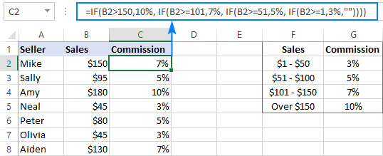
If we placed the conditions in the reverse order, from the bottom up, the results would be all wrong because our formula would stop after the first logical test (B2>=1) for any value greater than 1. Let's say, we have $100 in sales - it is greater than 1, so the formula would not check other conditions and return 3% as the result.
If you'd rather arrange the conditions from low to high, then use the "less than" operator and evaluate the "lowest" condition first, then the "second lowest", and so on:
=IF($B2<1, 0%, IF($B2<51, 3%, IF($B2<101, 5%, IF($B2<=150, 7%, 10%))))
As you see, it takes quite a lot of thought to build the logic of a nested IF statement correctly all the way to the end. And although Microsoft Excel allows nesting up to 64 IF functions in one formula, it is not something you'd really want to do in your worksheets. So, if you (or someone else) are gazing at your Excel nested IF formula trying to figure out what it actually does, it's time to reconsider your strategy and probably choose another tool in your arsenal.
For more information, please see Excel nested IF statement.
Nested IF with OR/AND conditions
In case you need to evaluate a few sets of different conditions, you can express those conditions using OR as well as AND function, nest the functions inside IF statements, and then nest the IF statements into each other.
Nested IF in Excel with OR statements
By using the OR function you can check two or more different conditions in the logical test of each IF function and return TRUE if any (at least one) of the OR arguments evaluates to TRUE. To see how it actually works, please consider the following example.
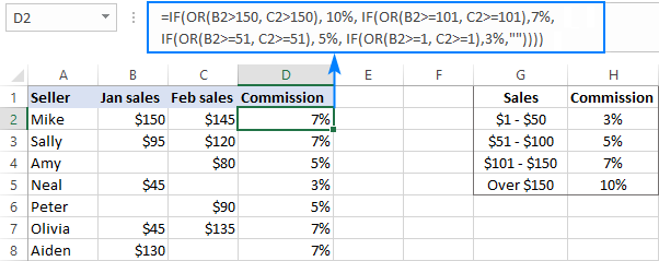
Supposing, you have two columns of sales, say January sales in column B and February sales in column C. You wish to check the numbers in both columns and calculate the commission based on a higher number. In other words, you build a formula with the following logic: if either Jan or Feb sales are greater than $150, the seller gets 10% commission, if Jan or Feb sales are greater than or equal to $101, the seller gets 7% commission, and so on.
To have it done, write a few OF statements like OR(B2>150, C2>150) and nest them into the logical tests of the IF functions discussed above. As the result, you get this formula:
=IF(OR(B2>150, C2>150), 10%, IF(OR(B2>=101, C2>=101),7%, IF(OR(B2>=51, C2>=51), 5%, IF(OR(B2>=1, C2>=1), 3%, ""))))
And have the commission assigned based on the higher sales amount:
For more formula examples, please see Excel IF OR statement.
Nested IF in Excel with AND statements
If your logical tests include multiple conditions, and all of those conditions should evaluate to TRUE, express them by using the AND function.
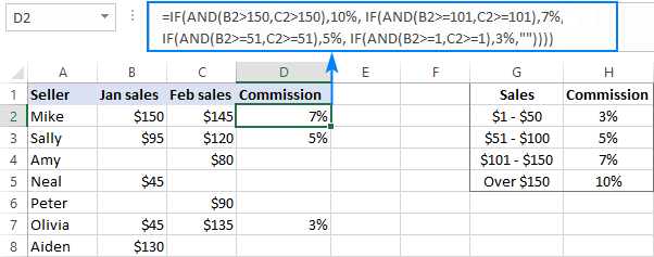
For example, to assign the commissions based on a lower number of sales, take the above formula and replace OR with AND statements. To put it differently, you tell Excel to return 10% only if Jan and Feb sales are greater than $150, 7% if Jan and Feb sales are greater than or equal to $101, and so on.
=IF(AND(B2>150, C2>150), 10%, IF(AND(B2>=101, C2>=101), 7%, IF(AND(B2>=51, C2>=51), 5%, IF(AND(B2>=1, C2>=1), 3%, ""))))
As the result, our nested IF formula calculates the commission based on the lower number in columns B and C. If either column is empty, there is no commission at all because none of the AND conditions is met:
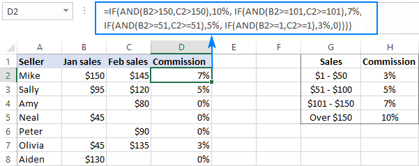
If you'd like to return 0% instead of blank cells, replace an empty string (''") in the last argument with 0%:
=IF(AND(B2>150, C2>150), 10%, IF(AND(B2>=101, C2>=101), 7%, IF(AND(B2>=51, C2>=51), 5%, IF(AND(B2>=1, C2>=1), 3%, 0%))))
More information can be found here: Excel IF with multiple AND/OR conditions.
VLOOKUP instead of nested IF in Excel
When you are dealing with "scales", i.e. continuous ranges of numerical values that together cover the entire range, in most cases you can use the VLOOKUP function instead of nested IFs.
For starters, make a reference table like shown in the screenshot below. And then, build a Vlookup formula with approximate match, i.e. with the range_lookup argument set to TRUE.
Assuming the lookup value is in B2 and the reference table is F2:G5, the formula goes as follows:
=VLOOKUP(B2,$F$2:$G$5,2,TRUE)
Please notice that we fix the table_array with absolute references ($F$2:$G$5) for the formula to copy correctly to other cells:
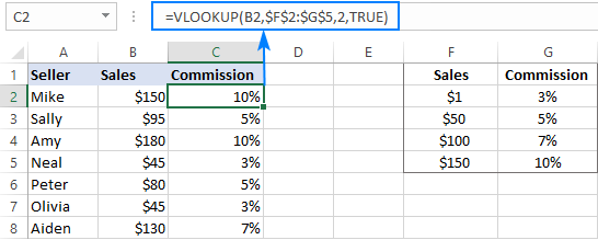
By setting the last argument of your Vlookup formula to TRUE, you tell Excel to search for the closest match - if an exact match is not found, return the next largest value that is smaller than the lookup value. As the result, your formula will match not only the exact values in the lookup table, but also any values that fall in between.
For example, the lookup value in B3 is $95. This number does not exist in the lookup table, and Vlookup with exact match would return an #N/A error in this case. But Vlookup with approximate match continues searching until it finds the nearest value that is less than the lookup value (which is $50 in our example) and returns a value from the second column in the same row (which is 5%).
But what if the lookup value is less than the smallest number in the lookup table or the lookup cell is empty? In this case, a Vlookup formula will return the #N/A error. If it's not what you actually want, nest VLOOKUP inside IFERROR and supply the value to output when the lookup value is not found. For example:
=IFERROR(VLOOKUP(B2, $F$2:$G$5, 2, TRUE), "Outside range")
Important note! For a Vlookup formula with approximate match to work correctly, the first column in the lookup table must be sorted in ascending order, from smallest to largest.
For more information, please see Exact match VLOOKUP vs. approximate match VLOOKUP.
IFS statement as alternative to nested IF function
In Excel 2016 and later versions, Microsoft introduced a special function to evaluate multiple conditions - the IFS function.
An IFS formula can handle up to 127 logical_test/value_if_true pairs, and the first logical test that evaluates to TRUE "wins":
In accordance with the above syntax, our nested IF formula can be reconstructed in this way:
=IFS(B2>150, 10%, B2>=101, 7%, B2>=51, 5%, B2>0, 3%)
Please pay attention that the IFS function returns the #N/A error if none of the specified conditions is met. To avoid this, you can add one more logical_test/value_if_true to the end of your formula that will return 0 or empty string ("") or whatever value you want if none of the previous logical tests is TRUE:
=IFS(B2>150, 10%, B2>=101, 7%, B2>=51, 5%, B2>0, 3%, TRUE, "")
As the result, our formula will return an empty string (blank cell) instead of the #N/A error if a corresponding cell in column B is empty or contains text or negative number.
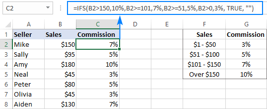
Note. Like nested IF, Excel's IFS function returns a value corresponding to the first condition that evaluates to TRUE, which is why the order of logical tests in an IFS formula matters.
For more information, please see Excel IFS function instead of nested IF.
CHOOSE instead of nested IF formula in Excel
Another way to test multiple conditions within a single formula in Excel is using the CHOOSE function, which is designed to return a value from the list based on a position of that value.
Applied to our sample dataset, the formula takes the following shape:
=CHOOSE((B2>=1) + (B2>=51) + (B2>=101) + (B2>150), 3%, 5%, 7%, 10%)
In the first argument (index_num), you evaluate all the conditions and add up the results. Given that TRUE equates to 1 and FALSE to 0, this way you calculate the position of the value to return.
For example, the value in B2 is $150. For this value, the first 3 conditions are TRUE and the last one (B2 > 150) is FALSE. So, index_num equals to 3, meaning the 3rd value is returned, which is 7%.
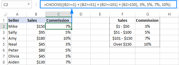
Tip. If none of the logical tests is TRUE, index_num is equal to 0, and the formula returns the #VALUE! error. An easy fix is wrapping CHOOSE in the IFERROR function like this:
=IFERROR(CHOOSE((B2>=1) + (B2>=51) + (B2>=101) + (B2>150), 3%, 5%, 7%, 10%), "")
For more information, please see Excel CHOOSE function with formula examples.
SWITCH function as a concise form of nested IF in Excel
In situations when you are dealing with a fixed set of predefined values, not scales, the SWITCH function can be a compact alternative to complex nested IF statements:
The SWITCH function evaluates expression against a list of values and returns the result corresponding to the first found match.
In case, you'd like to calculate the commission based on the following grades, rather than sales amounts, you could use this compact version of nested IF formula in Excel:
=SWITCH(C2, "A", 10%, "B", 7%, "C", 5%, "D", 3%, "")
Or, you can make a reference table like shown in the screenshot below and use cell references instead of hardcoded values:
=SWITCH(C2, $F$2, $G$2, $F$3, $G$3, $F$4, $G$4, $F$5, $G$5, "")
Please notice that we lock all references except the first one with the $ sign to prevent them from changing when copying the formula to other cells:
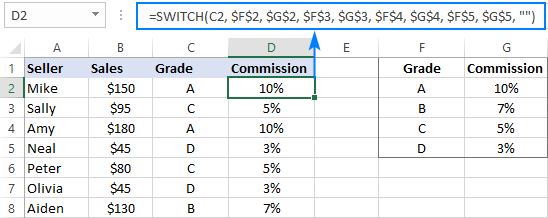
Note. The SWITCH function is only available in Excel 2016 and higher.
For more information, please see SWITCH function - the compact form of nested IF statement.
Concatenating multiple IF functions in Excel
As mentioned in the previous example, the SWITCH function was introduced only in Excel 2016. To handle similar tasks in older Excel versions, you can combine two or more IF statements by using the Concatenate operator (&) or the CONCATENATE function.
For example:
=(IF(C2="a", 10%, "") & IF(C2="b", 7%, "") & IF(C2="c", 5%, "") & IF(C2="d", 3%, ""))*1
Or
=CONCATENATE(IF(C2="a", 10%, ""), IF(C2="b", 7%, ""), IF(C2="c", 5%, "") & IF(C2="d", 3%, ""))*1
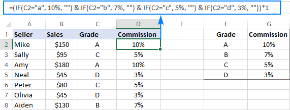
As you may have noticed, we multiply the result by 1 in both formulas. It is done to convert a string returned by the Concatenate formula to a number. If your expected output is text, then the multiplication operation is not needed.
For more information, please see CONCATENATE function in Excel.
You can see that Microsoft Excel provides a handful of good alternatives to nested IF formulas, and hopefully this tutorial has given you some clues on how to leverage them in your worksheets. To have a closer look at the examples discussed in this tutorial, you are welcome to download our sample workbook below. I thank you for reading and hope to see you on our blog next week!
Practice workbook for download
Excel nested If statement - examples (.xlsx file)
 by
by
226 comments
I need a formula if A1 is greater the or equal to 15 December 2019 or lesser then 14 March 2020 and if A2 says listed then say Yes if not say no or if A1 is greater then or equal to 15 March 2020 then say Yes.
Hello Bharath!
If I understand your task correctly, please try the following formula:
=IF(AND(A1 > = DATE(2019,12,15),A1 < = DATE(2020,3,14),A2="listed"),"YES",IF(A1 > = DATE(2020,3,15),"YES","NO"))
I hope it’ll be helpful.
1)If= first date of period all floor commission 2%
2)If=second date of period
lower floor commission 3% ,
middle floor commission 3.5%
Higher floor commission 4%
3)If = third date of period
Lower floor commission 2%
Middle floor commission 2.5%
Higher floor commission 3%
*(Date of periods
(1) 29-09-2019 to 02-02-2020
(2) 03-02-2020 to 29-02-2020
(3) 01-03-2020 to 30-03-2021)*
Can you please help any formula to get correct commission %
Please help it's very urgent....
Please help me!!!
I want to use an IF Command, but I want it in such a way that it fetches another IF Statement from a totally different Cell...
How do I do it?
Hello Abubakar!
If I understand your task correctly, the following formula should work for you:
=IF(C1,1,0)
in cell C1 write down the formula
=IF(A1>0,TRUE,FALSE)
I hope it’ll be helpful.
Hello,
I would ask for your advice in choosing the easiest procedure for determining ratings testing physical ability to take data from two different cells that are related to gender (male or female) and age group (is different for men and women, and can be easily determined on the basis of age using nested IF functions). Therefore, it is necessary to include data relating to gender and age category in the test results to obtain a score which is also categorized as laid down norms. Pre grateful!
My apologies... it sent before I finished my question.
Over Amt Short Amt Retailer ID
351.20 25862
10.00 37586
10.00 67952
351.20 25862
I would like to have the formula highlight amounts in red that are the same between Over Amt (col C) and short Amt (col D), but ONLY if the Retailer IDs (col E) are the same. As you can see here, the 351.20 amounts have the same retailer ID, but the 10.00 amounts do not. Any help you can give would be appreciated.
Thank you!
Chris
Good morning. I'm trying to figure out how to do the following:
Over Amt Short Amt Retailer ID
351.20
I NEED A ONE FORMULA FOR THIS:
I WANT TO WRITE "A" IN 2 CELLS AUTOMATICALLY IF WE BOOK AN APPOINTMENT FOR SERVICE "A"- 1 HOUR
AND TO WRITE "B" IN 2 CELLS AUTOMATICALLY IF WE BOOK AN APPOINTMENT FOR SERVICE "B" - 1 HOUR
AND TO WRITE "C" IN 4 CELLS AUTOMATICALLY IF WE BOOK AN APPOINTMENT FOR SERVICE "C" - 2 HOURS
AND TO WRITE "D" IN 3 CELLS AUTOMATICALLY IF WE BOOK AN APPOINTMENT FOR SERVICE "D" - 1.5 HOURS
PLEASE NOTE THAT THE ONE CELL MEAN 30 MINS.
I have a table of information. In the D column I have multiple products with various units of measure (g, mm, ml, kg, etc) I am attempting to build a formula that searches for the specific unit of measure and populates a new column with only that unit. Eg:
Column B3 information : DEN BRAVEN ACRYLIC BEECH/ OAK 280ml
Information I want the formula to find and place into column D "ml"
I have tried building a multiple IF but I it only identifies the first range of data successfully. The moment the Formula gets to a different unit of measure then it returns a #VALUE! issue.
Column B4 Data that the formula has issues with : ALCOLIN WOODFILLER OREGAN PINE 200g
Here is a copy of the IF:
=IF(FIND("ml";B3;1);"ml";IF(FIND("g";B3;1);"g";IF(FIND("m";B3;1);"m";"no")))
Could anyone give me some pointers?
A1 value is Male or Female
B2 Value is 10000 or 5000 or 15000 or 30000
in C2 result want if male is greater than 10000 then 200 or greater than 7500 then 175 or 0
or C2 result want if Female is greater than 10000 then 200 or 0
SOS, I am totally lost here.
I have 5 colons I need to take in my formula, with a total of 4 conditions and I need to calculate the following:
IF and and Then
condition1 D1460 G14=0 P14=0 =D14*$L$10
condition3 D14+G140 G14=<60 P14=Y D14*$L$10+$M$9
- and in all other cases it should be D14+G14
How do I get them all in one field and make excel calculate the result with all those parameters? Is it possible at all?
I tried with: IF((AND(D1460, G14=0), D14*$L$10, IF(D14+G14<=59, $M$9, IF((AND(G14=<60, P14=J), D14*$L$10+$M$9, D14+G14))))
But the formula is obviously wrong :-(
Since I am a linguist and the last time I had maths was in 1983, you can understand my confusion...
Many thanks!
Hi
I have to update the three different states professional tax values (PT) in column B based on the Column A (Salary) & Column C (states). state wise & Salary wise PT slab given below. I tried with if condition. It is throwing me an error. Can you help
Col A Col B Col C
Salary PT State TN PT Slab
1800 KL 12501 208.00
5500 KL
6000 KL KA PT Slab
6500 TN 0-15000 0
7500 TN >150001 200
7600 KL
8600 TN KL PT Slab
9000 TN 20834 208
25000 KA
I have a table with values, no text. The data look something like this
0.00 0.51 1.01 0.00 1.43
0.82 2.48 5.40 1.96 7.75
0.39 0.00 0.00 0.93 0.00
I need to present these values in four categories:
0 [presenting as 0]
>0 and <0.05 [presenting as =0.05 and =1 [presenting as the actual value]
I have not found a way for IFS to test against a range of values within a single unit of the function, as the old AND function used to enable in IF statements. Is this possible?
A chunk of the four categories got erased. Here are the categories, again:
0 [presenting as 0]
>0 and <0.05 [presenting as 0.04999 and 0.99999 [presenting as the actual value]
Thank you for better understand the if forula
I can’t figure out how to write this...the cell that I’m evaluating is a %
The formula I’ve tried: IF(B17≥65,"THRIVING",IF(B17≥50,"Ahead Of The Curve",IF(B17>35,"TURBULANT","Making Ends Meet")))
Criteria: 66+% = Thriving,
51-65% = Ahead Of The Curve,
36-50% = Making Ends Meet,
0-35% = Turbulent
One cell I’m evaluating has a value of 45%, another of 88%...the formula says both are Making Ends Meet
Can you help me?
HI Donna,
I thing this will you.
IF(A11>=66%,"THRIVING","")&IF(A11<=65%,"Ahead Of The Curve","")&IF(A11<=50%,"Making Ends Meet","")&IF(A11<=35%,"TURBULENT","")
169 #N/A
169 #N/A
169 #N/A
169 Punjab National Bank
169 #N/A
169 #N/A
i want to have punjab national bank in all the other places where it is #N/A. please share logic to write in other column
I need a formula for excel -
If (Salary<=13000) Then 9617 Else 12022 Elseif(Salary<=24000) Then 15100 ElseiF(salary<=30000) Then (Basic*0.45)
Help me
Sub Value()
Dim Salary As Integer
Dim Basic As Double
Basic = Cells(?, "?")
Salary = Cells(?, "?")
If Salary < 13001 Then
Cells(?, "?") = 9617
ElseIf Salary < 24001 Then
Cells(?, "?") = 15100
ElseIf Salary < 30001 Then
Cells(?, "?") = Basic * 0.45
Else
Cells(?, "?") = 12022
End If
End Sub
I am trying to find a max value from a list which belongs to another range of data. For example, when I have a data: A=1, B=2, C=3, D=4, E=5. If the list contains A, C, D, the output should be 4 (the maximum value).
I made a formula that works (F column: A,B,C,D,E; G column: 1,2,3,4,5; J column: list)as below: =MAX(IF(F22:F29=J21,G22:G29),IF(F22:F29=J22,G22:G29),IF(F22:F29=J23,G22:G29),IF(F22:F29=J24,G22:G29))
But I wonder, if there is any way to make the formula simpler.
Please help. My Formula mentioned below is working correctly.
=IF(I4>=9000, 2%, IF(I4>7500,1.75%, IF(I4>6000, "1.5%", IF(I4>4000, "1%", IF(I4=9000, 2%, IF(I4>7500,1.75%, IF(I4>6000, "1.5%", IF(I4>4000, "1%", IF(I4<4000, "0")))))), "0")
Thank you - this was extraordinarily helpful! The IF & IF & IF was exactly what I needed to make my column work properly. I used it in Google Sheets and it worked like a charm!
Afternoon, looking for some help with trending some date with date ranges. Have a data set with a lot of fluid data from multiple people and downloads. I need to 'Snap shot' the data in specific cells to track progress quickly for a trending report week on week. Complete a large search on the net but it I can not find anything the help with my problem. My current formula looks back at last weeks results which is misleading the data. Currently I have to manually over write the formula result each week manually so the data is retained and not re calculated, or over written. Any help appreciated..
hi, i have 3 different if formulas that works when entered separately. However, when i tried to combine them, the result shows "FALSE".
=IF(E3="PREVIEW 1",IF(N3>=11,30,IF(AND(N3>=10,N3=9,N3=12,30,IF(AND(N3>=11,N3=10,N3=14,30,IF(AND(N3>=13,N3<14),24,IF(N3=13,18,""))))))))))))
Please help me get the formulae for the below Ms excel problem. I need the card rate to appear automatically on the 4th column when the amount of Fixed Deposit (in millions), period of fixing (in days) & interest offered (%) is given. The card rates are given below.
FD(Mns) Days Int Offered(%) Card Rate (%)
2.65 31 7.50
11.34 91 7.50
64.21 181 8.00
178.58 365 8.75
CARD RATE
Days 10Mn50 Million
30 to 90 6.00 6.50 7.00
90 to 180 6.50 7.00 7.25
181 to 364 7.00 7.25 7.75
365 to 730 7.25 7.75 8.25
'=IF(AND(F9>0,F9=11,F9<=15),30,IF(F9<15,25,0)))
=IF(AND(F9>0,F9=11,F9<=15),30,IF(F9<15,25,0)))
@Nishith Rana try:
=IF(AND(F9>0,F9=11,F9<=15),30,IF(F9<15,25,0)))
=IF(0<F9<=10,45,IF(11<=F9<=15,30,IF(15<F9,25,0)))
THIS WONT WORK. HOW TO CORRECT THIS??
I run a badminton booking spreadsheet with 7 named players (as column headings in row 2) and I want to identify the first 4 people who have said "YES" (in row 3), working from the left. I have nested IFs, but I want to stop trying after I have achieved the 4th YES (because you can only get 4 player on a badminton court!).
This:
=CONCATENATE("This week it's ",
IF(C3="YES","me, ",""),
IF(D3="YES",$D$2,""),IF(D3="YES",", ",""),
IF(G3="YES",$G$2,""),IF(G3="YES",", ",""),
IF(I3="YES",$I$2,""),IF(I3="YES",", ",""),
IF(J3="YES",$J$2,""),IF(J3="YES",", ",""),
IF(K3="YES",$K$2,""),IF(K3="YES",", ",""),
IF(L3="YES",$L$2,""))
gives
"This week it's me, Roger, Sanath, Agnelo, Greg, Alec"
which is 6 names because José in column D had said "NO".
I would like the result to read
"This week it's me, Roger, Sanath, Agnelo".
I think the more gramatically correct
"This week it's me, Roger, Sanath and Agnelo"
might be too much of a challenge!
Any ideas please?
Hi Guy,
What if all the players reply in the affirmative? Will it be possIble to pick only four of them for a game without upsetting the others? If random selection sounds good to you, I can suggest applying a formula that will bring the names of those who want to take part (Step 1) and turning the values received into a 'Custom list' to delegate Ablebits' 'Random Generator' to take an unbiased decision (Step 2). If you like the idea, this is the formula which is needed in Step 1:
=IF($3:$3="YES", CHOOSE(1, $2:$2), "")
FYI =IF(G39="","",IF(J39=G39,"Contact individual",IF(M39="","",IF(M39<=J39,"Returned","Contact individual")))))
Hello please could you wizards advise on the following:
=IF(G40="","",IF(J40=G40,"Contact individual",IF(M40="","",IF(J40>=M40,"Returned","Contact individual")))))
I require a nest IF (if think)
I have three dates and three different document status outcomes depending on the sequence below.
If the issue date is is filled in only, then the status shall be "in circulation".
if there is now a document withdrawal date in the next cell that the is greater or equal to the issue date, the value shall be "Contact individual".
If the return date value is missing from the required cell then the status shall remain as "Contact individual", but if a date is entered into the withdrawal date cell the status then the status is to return "Returned"
Please Help Friends
I need to do an IF statement to get a range for:
Volumes Greater than and equal to 2,000,000
Volumes Less than 2,000,000 but greater than and equal to 200,000
Volumes less than 200,000 but greater than and equal to 500
Volumes less than and equal to 500
I just want to say thank you. I was able to create an if-choose on my excel thanks
Awesome article. I switched nested ifs for Lookup - made it so much easier. Also now I can go to the lookup table and change values without having to copy paste the formula again. Thanks....
I need help in defining the reorder level using "IF" or any other formula in excel
Column A = Shortage = 18500
Column B = MOQ = 5000
Column C = Reorder level = ?
I would like to calculate the reorder level as follows :-
(ie. Reorder level should be = to MOQ if shortage is less than MOQ
OR Reorder level should be 20000 if shortage is between 15001 & 20000
ie. Reorder level should be in multiples of MOQ but > shortage
Kindly confirm how to use "IF" formula or any other formula in excel
Tony,
You do not need an IF function for this.
Try:
=CEILING(shortage, 5000)
This will round your shortage number up to the next 5000.
K
Thanks a lot. it did work
Error in your explanation of the SWITCH function. Line 1, you use SWIFT. I expect you mean SWITCH. #yourewelcome
Of course, I meant SWITCH. Fixed, thank you!
I have a formula I am trying to use for Overbillings and underbillings, each a separate column. If I use one column the formula looks like this:
=IF([@[% Comp]]<30%,[@[Earned Cost]],[@[% Comp]]*[@[Contract Amount]])-[@Billed]
but I want it to give the result of zero if the answer to this in the overbillings is over zero. What do i add?
I am attempting to create a formula with IF statements.
Here it is:
G6 =TODAY() which inputs today's date.
J6 If "Yes" is selected
L6 will input TODAY()+7
=IF(J6="Yes",G6=TODAY()+7) the result will go into L6
Thank you
I am attempting to create a dynamic table where the value in one cell makes another equal a 3rd cell plus the data in another cell. So for example, =IF(F2=P7,G2+Q7,"-") I can get it to work with that one---but I need to nest that statement with 10+ others of the same type (=IF(f2=P8,G2+Q8) etc etc (pulling data from a table). I'm lost.
Not working. Please help please. I need to use 16 conditions for if statement but as you see, it is only 10 and not working. It said that "this formula uses more levels of nesting than you can use in the current file format". Anyone please.
Thanks!
=IF(S10>=95,20, IF(S10=94,19, if(s10=93,18, if(s10=92,17, if(s10=91,16, if(s10=90,15, if(s10=89,14, if(s10=88,13, if(s10=87,12, if(s10=86,11))))))))))
I know this is kind of late, but try this:
=IF(S10>=95,20, IF(and(S1085),s10-75,))
For some reason that did not format correctly. I will try it one more time:
=IF(S10>=95,20,IF(and(S10 85),s10-75,))
Can I use nested IF to do the following :
I have a column with three possibilities entered in the cells : ABC DEF GHI
the next column in the contagious cell needs a number based on the above so that :
ABC would be 123
DEF would be 456
GHI would be 789
Hi Bob,
Your formula may be as follows:
=IF(A2="ABC", 123, IF(A2="DEF", 456, IF(A2="GHI",789)))
Please have a look at Svetlana Cheusheva's article 'Excel nested IF statement - multiple conditions in a single formula' to learn more about the IF function.
I have 2 work sheets, the first one named Property 1 and the 2nd one named summery.
In the first sheet I have expenses listed by date, amount and category. the categories are Repairs,Labor,Materials,Transport,Advertising and Commission.
I would like to sum each category monthly (Jan,Feb.....) and display the total on the Summery sheet.
I'm trying to make a formula along the lines of if D3>= 2300 multiply by J3, once 2300 is exceed the difference should be multiplied by K3. Is this possible?
Rustin.
Your formula is missing the condition. If 'UTILITY Rates'!A2:A13 equal, larger, contains, etc
My formula wont work, can anyone see where I am going wrong?
=IF('UTILITY Rates'!A2:A13,'Utility Score Card'!C1,"'UTILITY Rates'!C2")
Hello. I have look different ways, but I'm running out of time to complete a project I'm working on. I have a table like this, is a changing pattern, so there is not actually a pattern, but there are some blank cells in between the text in Column A. In Column be I have tax names, which is just next. I need to be able to concatenate a formula with if or I don;t know to be able to concatenate tax names on the row with out blanks, I need to delete the blanks but have that information in every text
A B C
Text1 tax1 tax1,tax2
blank tax2 ------------
text2 tax1 tax1,tax2
blank tax2 --------------
text3 tax1 tax1
text4 tax1 tax1
text5 tax1 tax1
text6 tax1 tax1,tax2,tax3,tax4,tax5
blank tax2 --------
blank tax3 --------
blank tax4 ---------
blank tax5 -------
text7 tax1 tax1,tax2,tax3,tax4
blank tax2 ------------
blank tax3 ------------
blank tax4 -------------
text8 tax1 tax1
text9 tax2 tax2
text10 tax3 tax3,tax2
blank Tax2 ---------
test11 tax1 tax1
I'm having trouble with this formula. I have three conditions and they need to all be true to return "TRUE". If any are not true, it should return "FALSE". Here's what I've tried now, which does not work.
=IFS(C:C="CSD_SERVICES", "TRUE", (K:K=0,"TRUE", (O:O="","TRUE","FALSE")))
I've tried probably 25 different iterations but so far none returns the correct answer.
Hi,
It seems to me that any of the two formulas below can help you with your task:
=IF(AND(C:C="CSD_SERVICES", K:K=0, O:O=""), "TRUE", "FALSE")
=IFS(AND(C:C="CSD_SERVICES", K:K=0, O:O=""), "TRUE", TRUE, "FALSE")
Please note that the necessity of one more 'TRUE' in the second formula is dictated by the syntax that the Excel IFS function has. Please press 'F1' if you feel like looking into it.
if D4<=4,
true E4*50%,
False E4*100% but if
E45%, true E4*100%,false 5%
IF sentens:
About getting % when buying
Ih I by <= 4 pallets I´ll get 60%
If I by 5 but les than 9 pallets I'll get 60% and from his price I get ekstra 5 %
J=Amount of Pallets
L= My price (pallets times price pr. pallet)
M= 60 %
This works perfectly:
=IF(J6<=4;L6;L6-(IF(OR(J6=5;J6<=9);L6*(M6))))*(0,95)
My problem comes when I add this:
10 pallets but than 15 pallets I get 10 % (so first the 60 % and than an ekstra 10 after the first results.
Like this:
=IF(J6<=4;L6;L6-(IF(OR(J6=5;J6<=9);L6*(M6))))*(0,95);(IF(OR(J6=5;J6<=9);L6*(M6))))*(0,93);(IF(OR(J6=5;J6<=9);L6*(M6))))*(0,90)
I have a summary of invoices (positive) and credit notes (negative).
When I knock off against payment made it shows zero.
I am trying to make an if statement which would show:-
If zero - "-"
If more than .01 - "OS" (invoice)
If more than -.01 - "OS" (CN)
The aim is to filter what are the unpaid invoice and CN to generate
a payment proposal for those outstanding.
Thanks
I'm using a nested IF formula for conditional formatting and to evaluate if the date in a cell is equal to today =IF(I2=TODAY(),I2,IF(J2="NDA",J2,IF(J2="SDA",J2))). I want the formula to stop if the date in cell I2 is not equal today. The formula should stop at the first false argument however the formula evaluates all the arguments and returns a NDA which is the value in J2. I have evaluated the formula using Formula Auditing and I get a false value whether or not my first logical test is nested in an nested IF formula.
I have the following data in C7:
S123 - using formula will result in D7 as 80123
SA123 - using formula will result in D7 as 81123
E123 - using formula will result in D7 as 82123
EA123 - using formula will result in D7 as 83123
C123 - using formula will result in D7 as 84123
CA123 - using formula will result in D7 as 85123
U123 - using formula will result in D7 as 87123
UA123 - using formula will result in D7 as 86123
I tried to nest IF statements but excel is returning an error that maximum nesting is reached.
FORMULA:
=IF(LEFT(C7,2)="SA",CONCATENATE(81,RIGHT(C7,3)),IF(LEFT(C7,1)
="S",CONCATENATE(80,RIGHT(C7,3)),IF(LEFT(C7,2)="UA",CONCATENATE(87,RIGHT
(C7,3)),IF(LEFT(C7,1)="U",CONCATENATE(86,RIGHT(C7,3)),IF(LEFT(C7,2)
="CA",CONCATENATE(85,RIGHT(C7,3)),IF(LEFT(C7,1)="C",CONCATENATE(84,RIGHT
(C7,3)),"-"))))))
Dear Sir,
Kindly confirm one coloum are value 1-15, and secound Coloum value 15-30, if kindly confirm which sort out the value's of Below & uper.
& kindly confirm vlookup formulas fungtions.
I created a drop box of names in cell H67. I wanted my nested if statement to return some numbers and alphabets when a name is selected but it's not working.
Eg.
=IF(H67="M.ISAAC","000234-UMTP",IF(H67="D.MICHAEL","000678-UMPT",""))
The statement is not working. What am I doing wrong?
Do you offer classes online?
Hi!
Tell me what doesn't work. What result would you like to get? You can also find useful information in this article: How to compare two cells in Excel (string comparison).
Thanks for the reply.
When a name is selected from H67,
The result in H68 should be 000234-UMPT.
Hi!
Write the formula in H68. If the condition is true, get the desired result.