The tutorial explains the syntax of the Excel FIND and SEARCH functions and provides formula examples of advanced non-trivial uses.
In the last article, we covered the basics of the Excel Find and Replace dialog. In many situations, however, you may want Excel to find and extract data from other cells automatically based on your criteria. So, let's have a closer look at what the Excel search functions have to offer.
Excel FIND function
The FIND function in Excel is used to return the position of a specific character or substring within a text string.
The syntax of the Excel Find function is as follows:
The first 2 arguments are required, the last one is optional.
- Find_text - the character or substring you want to find.
- Within_text - the text string to be searched within. Usually it's supplied as a cell reference, but you can also type the string directly in the formula.
- Start_num - an optional argument that specifies from which character the search shall begin. If omitted, the search starts from the 1st character of the within_text string.
If the FIND function does not find the find_text character(s), a #VALUE! error is returned.
For example, the formula =FIND("d", "find") returns 4 because "d" is the 4th letter in the word "find". The formula =FIND("a", "find") returns an error because there is no "a" in "find".
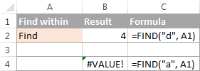
Excel FIND function - things to remember!
To correctly use a FIND formula in Excel, keep in mind the following simple facts:
- The FIND function is case sensitive. If you are looking for a case-insensitive match, use the SEARCH function.
- The FIND function in Excel does not allow using wildcard characters.
- If the find_text argument contains several characters, the FIND function returns the position of the first character. For example, the formula FIND("ap","happy") returns 2 because "a" in the 2nd letter in the word "happy".
- If within_text contains several occurrences of find_text, the first occurrence is returned. For example, FIND("l", "hello") returns 3, which is the position of the first "l" character in the word "hello".
- If find_text is an empty string "", the Excel FIND formula returns the first character in the search string.
- The Excel FIND function returns the #VALUE! error if any of the following occurs:
- Find_text does not exist in within_text.
- Start_num contains more characters than within_text.
- Start_num is 0 (zero) or a negative number.
Excel SEARCH function
The SEARCH function in Excel is very similar to FIND in that it also returns the location of a substring in a text string. Is syntax and arguments are akin to those of FIND:
Unlike FIND, the SEARCH function is case-insensitive and it allows using the wildcard characters, as demonstrated in the following example.
And here's a couple of basic Excel SEARCH formulas:
=SEARCH("market", "supermarket") returns 6 because the substring "market" begins at the 6th character of the word "supermarket".
=SEARCH("e", "Excel") returns 1 because "e" is the first character in the word "Excel", ignoring the case.
Like FIND, Excel's SEARCH function returns the #VALUE! error if:
- The value of the find_text argument is not found.
- The start_num argument is greater than the length of within_text.
- Start_num is equal to or less than zero.
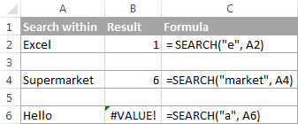
Further on in this tutorial, you will find a few more meaningful formula examples that demonstrate how to use SEARCH function in Excel worksheets.
Excel FIND vs. Excel SEARCH
As already mentioned, the FIND and SEARCH functions in Excel are very much alike in terms of syntax and uses. However, they do have a couple of differences.
1. Case-sensitive FIND vs. case-insensitive SEARCH
The most essential difference between the Excel SEARCH and FIND functions is that SEARCH is case-insensitive, while FIND is case-sensitive.
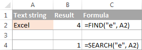
For example, SEARCH("e", "Excel") returns 1 because it ignores the case of "E", while FIND("e", "Excel") returns 4 because it minds the case.
2. Search with wildcard characters
Unlike FIND, the Excel SEARCH function accepts wildcard characters in the find_text argument:
- A question mark (?) matches one character, and
- An asterisk (*) matches any series of characters.
To see how it works on real data, consider the following example:
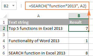
As you see in the screenshot above, the formula SEARCH("function*2013", A2) returns the position of the first character ("f") in the substring if the text string referred to in the within_text argument contains both "function" and "2013", no matter how many other characters there are in between.
Tip. To find an actual question mark (?) or asterisk (*), type a tilde (~) before the corresponding character.
Excel FIND and SEARCH formula examples
In practice, the Excel FIND and SEARCH functions are rarely used on their own. Typically, you would utilize them in combination with other functions such as MID, LEFT or RIGHT, and the following formula examples demonstrate some real-life uses.
Example 1. Find a string preceding or following a given character
This example shows how you can find and extract all characters in a text string to the left or to the right of a specific character. To make things easier to understand, consider the following example.
Supposing you have a column of names (column A) and you want to pull the First name and Last name into separate columns.
To get the first name, you can use FIND (or SEARCH) in conjunction with the LEFT function:
=LEFT(A2, FIND(" ", A2)-1)
or
=LEFT(A2, SEARCH(" ", A2)-1)
As you probably know, the Excel LEFT function returns the specified number of left-most characters in a string. And you use the FIND function to determine the position of a space (" ") to let the LEFT function know how many characters to extract. At that, you subtract 1 from the space's position because you don't want the returned value to include the space.
To extract the last name, use the combination of the RIGHT, FIND / SEARCH and LEN functions. The LEN function is needed to get the total number of characters in the string, from which you subtract the position of the space:
=RIGHT(A2,LEN(A2)-FIND(" ",A2))
or
=RIGHT(A2,LEN(A2)-SEARCH(" ",A2))
The following screenshot demonstrates the result:
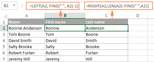
For more complex scenarios, such as extracting a middle name or splitting names with suffixes, please see How to split cells in Excel using formulas.
Example 2. Find Nth occurrence of a given character in a text string
Supposing you have some text strings in column A, say a list of SKUs, and you want to find the position of the 2nd dash in a string. The following formula works a treat:
=FIND("-", A2, FIND("-",A2)+1)
The first two arguments are easy to interpret: locate a dash ("-") in cell A2. In the third argument (start_num), you embed another FIND function that tells Excel to start searching beginning with the character that comes right after the first occurrence of dash (FIND("-",A2)+1).
To return the position of the 3rd occurrence, you embed the above formula in the start_num argument of another FIND function and add 2 to the returned value:
=FIND("-",A2, FIND("-", A2, FIND("-",A2)+1) +2)

Another and probably a simpler way of finding the Nth occurrence of a given character is using the Excel FIND function in combination with CHAR and SUBSTITUTE:
=FIND(CHAR(1),SUBSTITUTE(A2,"-",CHAR(1),3))
Where "-" is the character in question and "3" is the Nth occurrence you want to find.
In the above formula, the SUBSTITUTE function replaces the 3rd occurrence of dash ("-") with CHAR(1), which is the unprintable "Start of Heading" character in the ASCII system. Instead of CHAR(1) you can use any other unprintable character from 1 to 31. And then, the FIND function returns the position of that character in the text string. So, the general formula is as follows:
At first sight, it may seem that the above formulas have little practical value, but the next example will show how useful they are in solving real tasks.
Note. Please remember that the Excel FIND function is case-sensitive. In our example, this makes no difference, but if you are working with letters and you want a case-insensitive match, use the SEARCH function instead of FIND.
Example 3. Extract N characters following a certain character
To locate a substring of a given length within any text string, use Excel FIND or Excel SEARCH in combination with the MID function. The following example demonstrates how you can use such formulas in practice.
In our list of SKUs, supposing you want to find the first 3 characters following the first dash and pull them in another column.
If the group of characters preceding the first dash always contains the same number of items (e.g. 2 chars) this would be a trivial task. You could use the MID function to return 3 characters from a string, starting at position 4 (skipping the first 2 characters and a dash):
=MID(A2, 4, 3)
Translated into English, the formula says: "Look in cell A2, begin extracting from character 4, and return 3 characters".
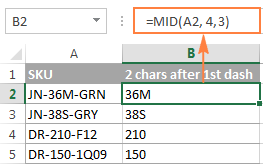
However, in real-life worksheets, the substring you need to extract could start anywhere within the text string. In our example, you may not know how many characters precede the first dash. To cope with this challenge, use the FIND function to determine the starting point of the substring that you want to retrieve.
The FIND formula to return the position of the 1st dash is as follows:
=FIND("-",A2)
Because you want to start with the character that follows the dash, add 1 to the returned value and embed the above function in the second argument (start_num) of the MID function:
=MID(A2, FIND("-",A2)+1, 3)
In this scenario, the Excel SEARCH function works equally well:
=MID(A2, SEARCH("-",A2)+1, 3)
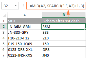
It's great, but what if the group of chars following the first dash contains a different number of characters? Hmm... this might be a problem:
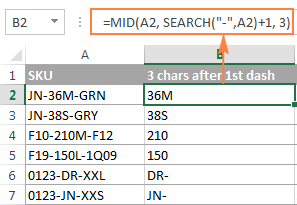
As you see in the above screenshot, the formula works perfectly for rows 1 and 2. In rows 4 and 5, the second group contains 4 characters, but only the first 3 chars are returned. In rows 6 and 7, there are only 2 characters in the second group, and therefore our Excel Search formula returns a dash following them.
If you wanted to return all chars between the 1st and 2nd occurrences of a certain character (dash in this example), how would you proceed? Here is the answer:
=MID(A2, FIND("-",A2)+1, FIND("-", A2, FIND("-",A2)+1) - FIND("-",A2)-1)
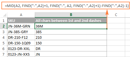
For better understanding of this MID formula, let's examine its arguments one by one:
- 1st argument (text). It's the text string containing the characters you want to extract, cell A2 in this example.
- 2nd argument (start_position). Specifies the position of the first character you want to extract. You use the FIND function to locate the first dash in the string and add 1 to that value because you want to start with the character that follows the dash: FIND("-",A2)+1.
- 3rd argument (num_chars). Specifies the number of characters you want to return. In our formula, this is the trickiest part. You use two FIND (or SEARCH) functions, one determines the position of the first dash: FIND("-",A2). And the other returns the position of the second dash: FIND("-", A2, FIND("-",A2)+1). Then you subtract the former from the latter, and then subtract 1 because you don't want to include either dash. As the result, you will get the number of characters between the 1st and 2nd dashes, which is exactly what we are looking for. So, you feed that value to the num_chars argument of the MID function.
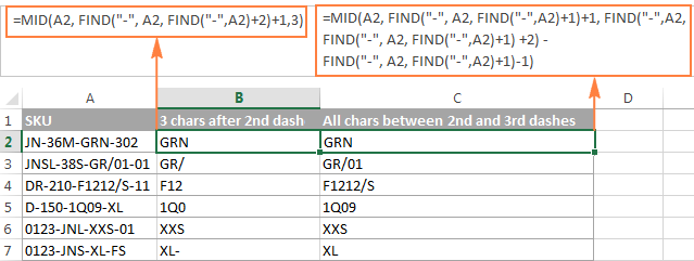
In a similar fashion, you can return 3 characters after the 2nd dash:
=MID(A2, FIND("-",A2, FIND("-", A2, FIND("-",A2)+1) +2), 3)
Or, extract all the characters between the 2nd and 3rd dashes:
=MID(A2, FIND("-", A2, FIND("-",A2)+1)+1, FIND("-",A2, FIND("-", A2, FIND("-",A2)+1) +2) - FIND("-", A2, FIND("-",A2)+1)-1)
Example 4. Find text between parentheses
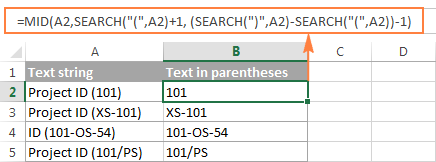
Supposing you have some long text string in column A and you want to find and extract only the text enclosed in (parentheses).
To do this, you would need the MID function to return the desired number of characters from a string, and either Excel FIND or SEARCH function to determine where to start and how many characters to extract.
=MID(A2,SEARCH("(",A2)+1, SEARCH(")",A2)-SEARCH("(",A2)-1)
The logic of this formula is similar to the ones we discussed in the previous example. And again, the most complex part is the last argument that tells the formula how many characters to return. That pretty long expression in the num_chars argument does the following:
- First, you find the position of the closing parenthesis:
SEARCH(")",A2) - After that you locate the position of the opening parenthesis:
SEARCH("(",A2) - And then, you calculate the difference between the positions of the closing and opening parentheses and subtract 1 from that number, because you don't want either parenthesis in the result:
SEARCH(")",A2)-SEARCH("(",A2))-1
Naturally, nothing prevents you from using the Excel FIND function instead of SEARCH, because case-sensitivity or case-insensitivity makes no difference in this example.
Hopefully, this tutorial has shed some light on how to use SEARCH and FIND functions in Excel. In the next tutorial, we are going to closely examine the REPLACE function, so please stay tuned. Thank you for reading!
 by
by
423 comments
Hi,
I would really appreciate if you can help me. I have a list of 150 popular words (A1: A150). I have a set of 500 customers' comments (B1: B500). I want to write a function that for each customer comment, excel searches for the occurrence of any of the 150 popular words (A1: A150) and returns the frequency of their occurrence in a cell in front of each customer.
For example, if I have 4 words (good, tasty, quite, fresh, like), and customer A said: "the meal was very tasty and fresh. I like the way food is presented. I also like the colours used in the place".
In this comment, tasty used 1 time; fresh used 1 time; like used twice.
I want the function to calculate the occurrence of these words as 4 times. I don't care about how many each word is repeated. I just need the total. I also want the function to be case insensitive since some customer might use capital case letters and other use lower case letters.
Many thanks
Hello!
Please try the following formula:
=SUM((LEN(A1)-LEN(SUBSTITUTE(A1,$D$1:$D$150,""))) / LEN($D$1:$D$150))
where
$D$1:$D$150 - list of 150 popular words
I hope it’ll be helpful.
Many thanks. It worked very well.
I also updated it to be case insensitive by
=SUM((LEN(A1)-LEN(SUBSTITUTE(UPPER(A1),UPPER($D$1:$D$150),""))) / LEN($D$1:$D$150))
Thanks again. Much appreciated
Currently looking to extract text within an individual cell, using a list that contains characters in a list I created. The text in the list ranges from A0-Z10 as this is what is within all those cells that I am trying to extract. So for example Cell B2 reads "John Anderson H0468582 Dr. James Dean" This is just an example as the placing of the middle set of characters isn't always consistent. So i am trying to extract the H0468582 based off there being a "H0" in the list I created (which sits within a different tab of the excel sheet) in to cell H2 for example.
I'm not sure if I explained it very well but if you can help then that would be great
Hello!
Please try the following formula:
=LEFT(MID(A1,IF(SUM(IFERROR(SEARCH(G1:G10,A1,1),"")) > 0,SUM(IFERROR(SEARCH(G1:G10,A1,1),"")),""),100), SEARCH(" ",MID(A1,IF(SUM(IFERROR(SEARCH(G1:G10,A1,1),"")) > 0,SUM(IFERROR(SEARCH(G1:G10,A1,1),"")),""),100),1))
G1:G10 - list ranges, no blanks.
I hope it’ll be helpful.
Dear Madam, I am searching a words content , an example
Searching "100A TP 50KA EU" from sheet-1 to sheet-2 "100A TP ACB 50KA FIXED LSI FRANCE EU"
Please help me to get suitable formula.
Hi,
You haven't written what result you want to get. To determine that the text was found, you can use the following formula
=IF(IFERROR(SEARCH("*"&SUBSTITUTE(A1," ","*")&"*",B1,1),"")>0,"Yes","No")
A1 is “100A TP 50KA EU”.
I hope it’ll be helpful.
=LEFT(C3;SEARCH("/3/";C3)-1)
=LEFT(C3;SEARCH("/2/";C3)-1)
=LEFT(C3;SEARCH("/1/";C3)-1)
how to sum up these three search criteria in one formula and when this value is missing to return the text to the cell
Hello!
If I got you right, the formula below will help you with your task:
=CONCAT(IFERROR(LEFT(C3,SEARCH({"/1/","/2/","/3/"},C3)-1),""))
I hope I answered your question. If something is still unclear, please feel free to ask.
Hi
need help to match number from 2 different columns and the result is true if matching for example in one column i have 12345 and that is randomly placed in the other column, so if column A and Column B has 12345 the result should be true or else it should be false
I am trying to make a department shift schedule where I list the start times and fill in names, then transfer the information to a standard schedule. For example, if Sue's name is in the first 3 cells, then she is scheduled for 6:30A, if in the next 3 cells, then 7:00A, etc. What function will give me a value based on which cell her name is in?
Hello! I need help expanding on the concept of finding text between parenthesis. I have a cell with lots of lines of text between parenthesis and I want to find all the instances of words between parenthesis in this single cell, not just the first one. How do I get the formula =MID(P2,SEARCH("",P2)-SEARCH("<",P2)-1) to repeat for the second, third, fourth instances etc. of text between parenthesis?
Hi,
I want to extract the Invoice Number from the column of comments with different texts.
So, the first check is whether the cell has an Invoice number, If yes, then I need to extract the 4 digit number from the text string.
Please guide how I can do that.
Reverse - Standby Invoice 7286 posted twice
BNP Security - LND 11697 Receipt No 9613 - CHERRYBROOK for 13/9 - 31/10/19
BNP Security - LND 11697 Receipt No 9616 - NORWEST for 13/9 - 31/10/19
BNP Security - LND 11697 Receipt No 8252 - 129 Showground for Aug-19
Standby Invoice 7432 for Epping for May-20
Dear Sir ,
I have a list I need to do sorting based on 4 character or 5 digit from behind below are example.
appreciated if can help to sort or separate it will be easier rather than I do it manually
CB80W90D208 2
CB80W90P20 8
CBDEP0P16 2
CBDEP0P18 0
CBDEP2P18 223
CBDEP2P20 2
CBDGEAR100D208 0
CBDGEAR68D208 2
CBDST100D205 -9
CBDST100D208 8
CCOM100D205 4
Thanks
MilanoZalgiris
Real MadridFenerbahce
BarcelonaC.Zvezda
ValenciaMaccabi T.A.
NewcastleLondon Lions
Townsville (F)Bendigo (F)
Southside F. (F)Perth (F)
FlamengoCampo Mourao
PrometheusPAOK
Xarilaos T.AEK
Zielona GoraOstrow
Anwil W.A.Gdynia
Townsville (F)Bendigo (F)
Southside F. (F)Perth (F)
Sydney (F)Canberra (F)
WelsBC Vienna
Vienna DCA.Traiskirchen
OberwartKlosterneuburg
FlamengoCampo Mourao
Sao PauloFranca SP
MinasUnifacisa
BrasíliaPinheiros
KolinOstrava
ETHA E.Apop Paphos
Apoel N.E.N.Paralimni
OmoniaAEL Limassol
HermesAlkar
SkrljevoSibenik
ZabokZadar
HorsensHerlev W.
AmagerSvendborg
KobratKTP Basket
Helsinki S.UU-Korihait
Kaarinan U.B.Salon Vilpas
Mac.RishonB.Herzelia
L.RytasNeptunas
PrienaiPieno
FyllingenTromso
C.T.OsloNidaros J.
Asker AliensBaerums
EstudiantesUnicaja
Real BetisBilbao
ValenciaTenerife
ZaragozaBarcelona
Real MadridManresa
CantuVirtus Roma
PesaroR.Emilia
Fortitudo Bol.Virtus Bologna
TrentoVarese
BrindisiBrescia
MilanoVenezia
WurzburgHamburg
BayreuthMitteldeutscher
Alba BerlinBonn
Bayern M.Ludwigsburg
CrailsheimBamberg
IraklisPeristeri
LavriouIonikos N.
PanathinaikosKolossos
Dabrowa G.S.Wroclaw
StargardStarogard G.
BrasíliaPinheiros
Hi. Can anyone help me with a formula or vba to split these strings by the continuous middle continuous substing it contains? eg. Dabrowa G.S.Wroclaw in Dabrowa G.S. - Wroclaw. THX
My post may be neither necessary nor useful, just my subjective feedback..
Nevertheless, I need to thank Svetlana very much for the well-arranged, almost analytical tutorials, which have helped me a lot in my work, as well as this one right now.
Thanks a lot, Kind Regards.
Hi Jaroslav,
Thank you so much about your kind words about my work. I'm delighted to hear that our tutorials are useful to you!
Hi,
I would really appreciate if you can help me. I have a list of 150 popular words (A1: A150). I have a set of 500 customers' comments (B1: B500). I want to write a function that for each customer comment, excel searches for the occurrence of any of the 150 popular words (A1: A150) and returns the frequency of their occurrence in a cell in front of each customer.
For example, if I have 4 words (good, tasty, quite, fresh, like), and customer A said: "the meal was very tasty and fresh. I like the way food is presented. I also like the colours used in the place".
In this comment, tasty used 1 time; fresh used 1 time; like used twice.
I want the function to calculate the occurrence of these words as 4 times. I don't care about how many each word is repeated. I just need the total. I also want the function to be case insensitive since some customer might use capital case letters and other use lower case letters.
I used the following formula to count the frequency of one word, but can't adopt it to search for the 150 words in the word list I have in A1:A150
C1=ISNUMBER(SEARCH("like",B1))
I really appreciate your help.
I would really appreciate if you can help me with this request. I am struggling to work it out.
I have a query where I need to find any punctuation characters in a list of names (where they have accidentally typed something wrong). It makes sense to repeat the formula for each character I am trying to find which is fine but all find and search formulas seem to only search one cell and I'd like to put a range in there. Is there something I can use to search the whole range? or even a way of making the LEN() formula search a range as that would do the job. thanks
Sir/Mam,
In excel, i have a bundle of statements(A2) and other cell i have specific values(B2) with pipelines as separators within the value. Now, what formula to be used to compare the specific values if present in the statement or not and the output to highlight the value in the specific cell - B2
Hello!
Your task is not completely clear to me. Please describe your problem in more detail. Include an example of the source data and the result you want to get. It’ll help me understand your request better and find a solution for you.
hi, i would like to extract data from 1 sheet to other sheet .Like example , status have 3 input there, that is completed, cancel, shipping , i wan extract all the data regarding shipping. but i just can get 1 data of shipping. how can i do with extract all data regarding it
Hello!
Please check out the following article on our blog, it’ll be sure to help you with your task: How to VLOOKUP multiple values in Excel with one or more criteria
Hope you’ll find this information helpful.
I had tried the method but it direct show with wrong
this is what i type :
=IFERROR(INDEX(orders!$A$2:A,SMALL(IF($A$16=orders!$B$2:B,ROW(orders!$A$2:A)-MIN(ROW())+1,""),ROW()-1)),"wrong")
Hello!
Unfortunately, without seeing your data it is impossible to give you advice.
I'm sorry, it is not very clear what result you want to get. Could you please describe your task in more detail and send us a small sample workbook with the source data and expected result to support@ablebits.com? Please shorten your tables to 10-20 rows/columns and include the link to your blog comment.
We'll look into your task and try to help.
The column AG contains the combination of below, need to separate seconds, minute, hour,day,week, months in different column.
0s
32m 14s
3h 21m 18s
1w 1d 12h 0m 28s
6d 18h 36m 50s
1mos 2w 2d 9h 6m 56s
please help me with formula
Hello!
To split a space-delimited text string to columns, use this instruction.
If you have any other questions, please don’t hesitate to ask.
Please refer my expected result in Excel, kindly assist me, alignment is not correct.
Resolution Time Months Weeks Days Hours Minutes Seconds
0s 0 0 0 0 0 0
13m 17s 0 0 0 0 13 17
1h 48m 15s 0 0 0 1 48 15
4d 9h 27m 40s 0 0 4 9 27 40
1w 6d 7h 24m 12s 0 1 6 7 24 12
6d 16h 17m 38s 0 0 6 16 17 38
6h 13m 34s 0 0 0 6 13 34
1w 6d 7h 24m 12s 0 1 6 7 24 12
9h 0m 0s 0 0 0 9 0 0
1mos 2w 2d 9h 6m 56s 1 2 2 9 6 56
Hello!
The formula below will do the trick for you:
=REPT("0 ",5-(LEN(SUBSTITUTE(TRIM(CONCAT(IF(ISNUMBER(--MID(H1,ROW($1:$93),1)), MID(H1,ROW($1:$93),1)," ")))," "," ")) - LEN(SUBSTITUTE(SUBSTITUTE(TRIM(CONCAT(IF(ISNUMBER(--MID(H1,ROW($1:$93),1)), MID(H1,ROW($1:$93),1)," ")))," "," ")," ","")))) & SUBSTITUTE(TRIM(CONCAT(IF(ISNUMBER(--MID(H1,ROW($1:$93),1)), MID(H1,ROW($1:$93),1)," ")))," "," ")
Divide the resulting text into columns, as I advised you earlier.
I'd recommend you to have a look at our Ablebits Tools - Split text tool that can help you split the text to columns. It is available as a part of our Ultimate Suite for Excel that you can install in a trial mode and check how it works for free.
tried the free tool, but not getting the expected result. Formula applied in one column, need to be in separate column.
Hi, Would like to ask you help for this scenario below:
For example I have this data below in a column, and I want to search for which rows have "John" only in their name.
1.Johnson New
2.Jane John
3.Earl John Watson
4.Amy Anne John
With the data in Row 1, it returns a value for it because it contains "John" in "Johnson" but I won't be needing that because I need only the "John" name.
How can I do this in a formula? Thanks!
adding more data:
5.John Watsons
6.John Johnsons
Hello!
To find an exact match of a word in the text, you can use this formula:
=IF((ISNUMBER(FIND($A$1&" ",A2))+ISNUMBER(FIND(" "&$A$1,A2))+($A$1=A2))>0,TRUE,"")
where cell A1 contains the word that we are looking for in the text.
I hope my advice will help you solve your task.
I read through your article and most of the questions but haven't found a way of removing multiple instances that occur in a single cell. When I import a data table of projects with employee names and occupations from our system the information comes into an Excel table with the project number as the row and the various occupations as the columns. The names are displayed with system generated characters and id numbers.
For example for project manager the name of Sue Smith shows in the table as Smith,Sue;#56789. For occupations with a single entry I can use left and search functions to remove the";#56789" using =LEFT(A1,SEARCH(";",A1)-1). The problem comes in when I get multiple people for a occupation. For example for engineer I may get Jones, John;#1234;#Trifuntov,Alexander;#789;#Sharashova,Natalia;#90. If I use the above formula all I get is Jones, John and the other names are truncated. I am looking to have it come up as Jones, John;Trifuntov, Alexander;Sharashova,Natalia I have tries using REPLACE and SUBSTITUTE but due to the varying number of people, length of names and id numbers I keep getting issues. Is there any way to use a find/search formulas?
Hello!
For your example text, you can use the formula
=SUBSTITUTE(SUBSTITUTE(SUBSTITUTE((CONCAT(IF(NOT(ISNUMBER(--MID(A1,ROW($1:$91),1))),MID(A1,ROW($1:$91),1),"")))," ",""),"#;#",""),";#","")
It removes from the text all numbers and extra characters "#" and ";"
Hope this is what you need.
I really appreciate your fast response. When I use the above formula I get an error. Maybe we can start simple and once I get that correct I can expand. Let's say
Jones, John;#1234;#Trifuntov,Alexander;#789;#Sharashova,Natalia;#90 is in cell A1
and I want to look like
Jones, John; Trifuntov,Alexander; Sharashova,Natalia in cell B1.
What would the formula be in cell B1?
Again thanks and I appreciate your patience!
Hello,
I would very much appreciate any suggestions/guidance to find a specific text, "Apple," in the middle and at the end where there is no space in a cell. (Yes.. I am sorry and am feeling bad to have to ask this ignorant question as I am a new user.)
Here's my formula to find the text "Apple" in the middle.
=MID(A1,FIND("#Apple",A1,1)+1,(FIND(";",A1,FIND("#Apple",A1)))-(FIND("#Apple",A1,1)+1))
Column A
A1 - 15;#Apple;#121;#Pears - Organic;#18;#Banana;#87;#Strawberry;#38;Cherry;#149;#Orange
A2 - 18;#Banana;#87;#Strawberry;#38;#Cherry;#15;#Apple;#121;#Pears - Organic
A3 - 16;#DragonFruit;#121;#Pears - Organic;#18;#Banana;#87;#Strawberry;#38;Cherry;#15;#Apple
Column B with the MID Formula
B1 - Apple
B2 - Apple
B3 - #VALUE <-- because Apple is at the end
I need a formula that would get both middle and end....
Appreciate any suggestions/guidance.
Kind regards,
Miko
Hello Miko!
If you just need to extract "Apple" from the text, then you can just take 5 characters:
=MID(A1,FIND("#Apple",A1,1)+1,5)
I hope this will help, otherwise please do not hesitate to contact me anytime.
I cannot thank you enough. You saved hours of my time to prepare a weekly report out of crude SharePoint datadump.
Gratefully,
Miko
Hi,
I would like to search for a specifik text within a column. Example: If a cell cointains: "The upper side. System:20 Tag:20A-VA004" I would like to copy the tag number (Tag:20A-VA004) to a new cell, both tag written TAG, tag: and Tag. I have tried the formula =TRIM(LEFT(SUBSTITUTE(MID(C12;FIND("Tag:";C12);LEN(C12));" ";REPT(" ";100));100)), but this does not include space and different writings. Can you please help?
Regards, Kristin
Hello!
If I understand your task correctly, to extract text starting at some position, use the formula
=MID(D1,SEARCH("tag",D1,1),LEN(D1)-SEARCH("tag",D1,1)+1)
I hope it’ll be helpful.
Hi,
I need to extract number from strings like:
#34224 some text
#43543543: some text
#34243-some text
#3423145
so number can be different in length and be followed by space OR semicolon OR dash OR do not have any character after.
the formula that I have for the third case is =IFERROR(NUMBERVALUE(IF(SEARCH("#";[@Comment])=1;MID([@Comment];2;SEARCH("-";[@Comment])-2);FALSE));0)
but how to modify it to include all 4 cases?
Good day! I am struggling to work on this one. I need to mark the 50th word in a paragraph with * (still with the whole paragraph, im not just gonna extract the 50th word out) but if it is equal or less then 50 words, then I can just copy the text as it is. How can I do this? Thank you for your help!
Hello!
If I understand your task correctly, to put * before the 50th word, use the formula
=IF(LEN(C1)-LEN(SUBSTITUTE(C1," ",""))<51,LEN(C1)-LEN(SUBSTITUTE(C1," ","")),SUBSTITUTE(C1," ","*",50))
I hope this will help
Respected Sirs,
Here I have a problem to solve
in a coloumn of name there are three or two words name
Ram Bahadur Gautam
sanjay Limbu
I need to extract only last sir name to another column and copy the formula
Thank your for your kindly assistance
Sanay limbu
Hello!
If I got you right, the formula below will help you with your task:
=TRIM(RIGHT(SUBSTITUTE(A1," ",REPT(" ",20)),20))
This will help to extract the last word from the text.
Hi Alex! Great tutorials! I lead a group of sales coaches which write their feedback in an excel sheet. I am trying to build a formula which searches a keyword or phrase within a paragraph and the word or phrase after it ( Ex. keyword:OPPORTUNITY: FACT FINDING) Then, I would keep track how many times the phrase after the keyword was used. Any thoughts?
Hello Juan!
I’m sorry but your task is not entirely clear to me.
Please describe your problem in more detail.Is the feedback written in several cells or in one? Include an example of the source data and the result you want to get. It’ll help me understand your request better and find a solution for you. Thank you.
Cell A1 contains the googlefinanceticker NASDAQ:TQQQ
Cell B1 should contain a Formula wich verifies if A1 contains a colon. If YES than got the name of the ticker.
The idea should be like this, but I have problems with combination of funktion and syntaxis.
=IF(ISNUMBER(FIND(":";P2));AA2=GOOGLEFINANCE(AP2;"PRICE");"ist kein googlefinanceID")
Any idea !!! Thanks in advance for your help,
Valentin
Hello Valentin,
If I've got your task correctly and you work in Google Sheets, here's how your formula should look like:
=IF(ISNUMBER(FIND(":",P2)),GOOGLEFINANCE(P2,"PRICE"),"ist kein googlefinanceID")
Please refer to the following article about the IF function in Google Sheets to learn the correct syntax: https://www.ablebits.com/office-addins-blog/if-function-google-sheets/
There's even a tool that can figure out the syntax for you.
i want to use =RİGHT operation and every word contain ")" for ex asdasdasd),asdasdewqd),uymjutynm), but thera are a so many blanks and i want to delete blanks and i want to assigned them a number for exam. asdasdasd) = 123 asdasdewqd)=432 uymjutynm)=564 , there are a few exist them and i want to convert to number to text with use a only 1 letter that ")" how can i figure out
i think if i use matlab it facilitate my works or complicate my works
sorry for my bad english
Hi,
I want your help in finding a formula where i can pull of data from multiple row - having multiple data in each cell - and the cell has some key identifier at there first to look out the data.
For e.g. In row Cell 1- 32:hshsjsjsbsvshh
Cell2: 32:shsjsjsjsjsjsjjs
Cell3: 67:hwhsshshshshsh
Cell4: 69:hshsshsusushsh
So in above example i want the data in next sheet from the cell which is started from '32:'
Hello!
You did not say exactly how you want to extract the data. Suppose the data needs to be combined. If I understand your task correctly, Merge cells by condition using the array formula
=CONCAT(IF(LEFT(E2:E10,3)="32:",E2:E10,""))
Press Ctrl + Shift + Enter so that array function to work.
We merged all the cells that start with "32:"
Hi Alex,
Thanks for your reply but here i don't want to merged the cell, I want to pull out the data start with 32: as it is in the other excel sheet.
Hope you understand my query.
hello!
I don't want to guess anymore. Explain what kind of data you wanted to get from Cell 1-32: hshsjsjsbsvshh ??
Write the expected result for each cell.
I think I've figured it out on my own. Thank you anyway for your help.
Hi,
I'm trying to write an equation in Excel that rounds using the following rules:
1. If the extra digit is less than 5, drop the digit.
2. If the extra digit is greater than 5, drop it and increase the previous digit by one.
3. If the extra digit is five, then increase the previous digit by one if it is odd; otherwise do not change the previous digit.
I feel like I'm close to a solution by using the IF(AND(Find line of commands but can't get it to come together properly. Could you please help?
Thanks so much,
John
Hello John!
The Find function is applied to the text. In this case, I assume that we have a number. Apply the IF function and rounding function.
=IF(MOD(INT(A30),2)=0,IF(A30-INT(A30)<=0.5,INT(A30),ROUND(A30,0)),ROUNDUP(A30,0))
Hope this is what you need.
Thank you so much for your response Alexander!
I tried that function but didn't have much success. Maybe if I give you an example that would help.
If I have a number like 0.20645 and I would like it rounded to four decimal places and be rounded down if the value in the fourth place is even and the fifth value is =5, in this case 0.20645 would be rounded to 0.2064. On the flip side of that I would still like a value like 0.20615 to be rounded to four places but rounded down if the fourth value is odd and =5. In other words 0.20615 would be rounded to 0.2062.
This is the equation I've tried without success: =IF(AND(ISODD(MID(H12,FIND(".",H12)+4,4)),MID(H12,FIND(".",H12)+5,4)="5"),ROUNDUP(H12,4),IF(AND(ISEVEN(MID(H12,FIND(".",H12)+4,4)),MID(H12,FIND(".",H12)+5,4)="5"),ROUNDDOWN(H12,4),ROUNDDOWN(H12,4)))
I have a column A with multiple cells having a common value.
I also have a column B with equal number of cells each having a unique value.
I want to do a FInd and Replace such that it finds the common value in each cell of Column A and replace it with the unique value of adjoining cell of column B,
See screenshot for more clarity - https://prnt.sc/t0ksyn
Hello!
I hope you have studied the recommendations in the above tutorial.The Find function can search in only one cell. I’m sorry but your task is not entirely clear to me. Could you please describe it in more detail? What does "common value in each cell of Column A" mean? In column A, all cells have the same values. If a value is written in a cell, then it can be changed either manually or using the VBA macro. Therefore, the values in column A, you cannot change the values using the formula. Explain in more detail what you want to do.Thank you!
Hello Sir, I need a Formula/Function to show variance with multiple criteria…
Function needs applied to E:E in examples below- if it is needed to add extra columns, we can. If it needs to be done in VBA form, we can do that as well.
A - FIND B:B WITHIN F:F
SEARCH ( B:B , F:F )
B - TAKE THE MINIMUM OF D:D, WHERE “A” CRITERIA MATCHES (MULTIPLE SKU WITH DIFFERENT PRICING)
MIN ( D3 : D11 )
C - AND THEN MULTIPLY THAT MINIMUM BY 1.25
MIN ( D3 : D11 ) * 1.25
D – TAKE THAT NEW NUMBER AND APPLY IT TO ALL ROWS IN COLUMN D WHERE “A” & “B” CRITERIA ARE TRUE
(not sure how to do this part)
RAW DATA
1 B C D E F
2 SKU MKT MARKET PRICE 25% VARIANCE SKUMKT
3 1234 CHINA 18.98 1234CHINA
4 1234 AUSTRALIA 18.98 1234AUSTRALIA
5 1234 USA 17.03 1234USA
6 9876 CHINA 17.11 9876CHINA
7 9876 AUSTRALIA 18.98 9876AUSTRALIA
8 9876 USA 18.28 9876USA
9 4567 CHINA 18.98 4567CHINA
10 4567 AUSTRALIA 18.98 4567AUSTRALIA
11 4567 USA 18.63 4567USA
WHAT IT SHOULD LOOK LIKE WHEN COMPLETE
1 B C D E F
2 SKU MKT MARKET PRICE 25% VARIANCE SKUMKT
3 1234 CHINA 18.98 21.29 1234CHINA
4 1234 AUSTRALIA 18.98 21.29 1234AUSTRALIA
5 1234 USA 17.03 21.29 1234USA
6 9876 CHINA 17.11 21.38 9876CHINA
7 9876 AUSTRALIA 18.98 21.38 9876AUSTRALIA
8 9876 USA 18.28 21.38 9876USA
9 4567 CHINA 18.98 23.29 4567CHINA
10 4567 AUSTRALIA 18.98 23.29 4567AUSTRALIA
11 4567 USA 18.63 23.29 4567USA
Am I not able to do a formula like what it is I am hoping for?
Hello!
I’m sorry but your task is not entirely clear to me. For me to be able to help you better, please describe your task in more detail. Please specify what you were trying to find, what formula you used and what problem or error occurred. Give an example the expected result.
It’ll help me understand it better and find a solution for you. Thank you.
We need a Formula/Function to show variance with multiple criteria…
Function needs applied to E:E in examples below.
We need to find the same SKU numbers (column B) that have multiple markets (column C), find the lowest price of that SKU between those markets(column D), and then multiply that lowest price by 25% and be entered in column E for all of the SKUs that match.
A - FIND B:B WITHIN F:F
SEARCH ( B:B , F:F )
B - TAKE THE MINIMUM OF D:D, WHERE “A” CRITERIA MATCHES (MULTIPLE SKU WITH DIFFERENT PRICING)
MIN ( D3 : D11 )
C - AND THEN MULTIPLY THAT MINIMUM BY 1.25
MIN ( D3 : D11 ) * 1.25
D – TAKE THAT NEW NUMBER AND APPLY IT TO ALL ROWS IN COLUMN D WHERE “A” & “B” CRITERIA ARE TRUE
(not sure how to do this part)
RAW DATA
1.B.....C..........D..............E.............F
2 SKU .MARKET.....MARKET PRICE. 25% VARIANCE. SKUMKT
3 1234 CHINA ......18.98 ........()...........1234CHINA
4 1234 AUSTRALIA ..18.98 .........()...........1234AUSTRALIA
5 1234 USA ........17.03 .......().............1234USA
6 9876 CHINA ......17.11..........().......... 9876CHINA
7 9876 AUSTRALIA ..18.98 .........()...........9876AUSTRALIA
8 9876 USA ........18.28..........().......... 9876USA
9 4567 CHINA ......18.98 .........()...........4567CHINA
10 4567 AUSTRALIA ..18.98.........().......... 4567AUSTRALIA
11 4567 USA ........18.63 ........()............4567USA
WHAT IT SHOULD LOOK LIKE WHEN COMPLETE
1.B.....C..........D..............E...............F
2 SKU .MARKET..... MARKET PRICE.. 25% VARIANCE ..SKUMKT
3 1234 CHINA ......18.98 .........21.29 .........1234CHINA
4 1234 AUSTRALIA ..18.98 .........21.29 .........1234AUSTRALIA
5 1234 USA ........17.03 .........21.29 .........1234USA
6 9876 CHINA ......17.11 .........21.38 .........9876CHINA
7 9876 AUSTRALIA ..18.98 .........21.38 .........9876AUSTRALIA
8 9876 USA ........18.28 .........21.38 .........9876USA
9 4567 CHINA ......18.98 .........23.29 .........4567CHINA
10 4567 AUSTRALIA .18.98 .........23.29 .........4567AUSTRALIA
11 4567 USA .......18.63 .........23.29 .........4567USA
Hello!
Your request goes beyond the advice we provide on this blog. This is a complex solution that cannot be found with a single formula. If you have a specific question about the operation of a function or formula, I will try to answer it.
HI FOrum,
If i need to extract text from intial and last name with no character break, how do i do it?
Hello!
I recommend to study this article. Then describe the problem in more detail. Please let me know in more detail what you were trying to find, what formula you used and what problem or error occurred. Give an example of the source data and the expected result. It’ll help me understand it better and find a solution for you. Thank you.
Hi Sir,
In one column i have a string from which i have to extract the exact unique code which starts with "ABCD" and followed by 4 numeral characters (Example-ABCD2345)
Example String-
Information: ABCD: Update for Application 1 (ABCD2140) Rel. 1.01
Expected output- ABCD2140
Solution- =IFERROR(MID(C3,FIND("(ABCD",C3),FIND(")",C3)-FIND("(ABCD",C3)),"NA")
The solution works for above String, but it fails in cases where any "(" comes before "(ABCD".
Example-(XYZ) external – Application 2 (ABCD2003) Rel. 1.02
Expected Output- ABCD2003
Could you help me get a common solution which works for both the cases.
Hello!
If I understand your task correctly, the following formula should work for you:
="ABCD"&MID(C3,FIND("(ABCD",C3,1)+5,4)
I hope this will help, otherwise please do not hesitate to contact me anytime.
I have a string of text, similar to the following: This well requires cleaning; Y; $2,000; WB Abandonment; Y; $12,000; Other; N; $5,000.
I'd like to use a formula to search the string and if "WB Abandonment; Y;" is in the string it would return "$12,000". If "WB Abandonment; Y;" is not in the string, it returns blank. I'm struggling with the mid search formula since the various lines of text have a different number of components the well requires. Any help you can provide would be greatly appreciated.
Hello!
If I understand your task correctly, the following formula should work for you:
=IF(IFERROR(SEARCH("WB Abandonment; Y;",A1,1),0) > 0,"$ 12,000","")
I hope this will help, otherwise please do not hesitate to contact me anytime.
Sorry, I wasn't clear. The value isn't always $ 12,000. I'm looking to return the value that follows "WB Abandonment; Y;".
Hello Sue!
To get all the text after phrase “WB Abandonment; Y;”, use the formula
=IF(IFERROR(SEARCH("WB Abandonment; Y;",A1,1),0)>0, MID(A1,SEARCH("WB Abandonment; Y;",A1,1)+19,100),"")
If you wrote exactly what you want to receive, we would solve your problem faster.
Unfortunately this formula returns all the text after "WB Abandonment; Y;". I'm hoping to be able to only pull the $ amount after "WB Abandonment; Y;" and before the next ;.
Hi sir,
I have a question, my question is that the way we have used the left function with find ,same way we can't use the right function with find to get the last name.
Hi Alexander,
Thank you for your post. I have been unable to find any information to help me with my issue - perhaps you can help?
I have a text string in column L. Within this text string I can find a series of alternatives (which are contained in the OR brackets below). I've tried to simplify a heavy, clunky formula (1) to a more elegant (2), but (2) isn't working - it's not returning any values even if I know the value is contained in column L.
(1) Monster: =IFERROR(IFERROR(IFERROR(IFERROR((IFERROR(MID(L2,FIND("DPTO",L2),50),MID(L2,FIND("CASA ",L2),50))),(MID(L2,FIND("LOC ",L2),50))),(MID(L2,FIND("OF",L2),50))),(MID(L2,FIND("PARC",L2),50))),(MID(L2,FIND("DEPT",L2),50)))
(2) Failed attempt to simplify:
=MID(L2,FIND(OR("DPTO","CASA ","DEPT","LOC ","OF","PARC"),L2),50)
Am I doomed to clunkiness? Or am I making a silly mistake?
Thanks in advance!
Hello Alex!
For me to be able to help you better, please describe your task in more detail. Do you want to derive these values using a formula, or simply specify TRUE or FALSE, or derive some part of the cell from column L? What result should your formula return? Please let me know in more detail what you were trying to find, what problem or error occurred. It’ll help me understand it better and find a solution for you. Thank you.
The result of the formula should be the string text starting from the position found by the FIND formula (when it finds any of the alternatives included in the OR function brackets in equation 2) and the following 50 characters (which is why the MID formula is there).
Please let me know if you need more information!
Hello Alex!
If I understand your task correctly, the following formula should work for you:
=MID(L2,SMALL(IFERROR(FIND({"DEPT","CASA","OF","PARC"},L2,1),""),1),50)
I hope this will help, otherwise please do not hesitate to contact me anytime.
Unfortunately it doesn't work. I had previously tried putting an array in FIND but that didn't work either. Even just =FIND({"DEPT","CASA","OF","PARC"},L2,1) returns a #VALUE error instead of a place number.
The source string has a mix of text, numbers and blank spaces, General format, if that helps at all.
Hello Alex!
My formula works according to your explanation. Give an example of the data in cell L2 and the result you want to get. Explain what exactly the formula does not work in. Perhaps I misunderstood you. Or you didn’t say anything.
Your FIND formula will not work, because it does not handle the event when the value is not found.
OK so here's an example.
Cell L has this: AVENIDA DEL VALLE S/N ALGARROBOS 4B CASA 21B
Your formula: =MID(L2,SMALL(IFERROR(FIND({"DEPT","CASA","OF","PARC"},L2,1),""),1),50)
Is giving me this: #VALUE
When I need it to give this: CASA 21B
i.e. return the string from the position found by the FIND formula.
Hello Alex!
I copied the formula from your post:
=MID(L2,SMALL(IFERROR(FIND({"DEPT","CASA","OF","PARC"},L2,1),""),1),50)
I inserted text into cell L2:
AVENIDA DEL VALLE S/N ALGARROBOS 4B CASA 21B
And you won’t believe it - everything works for me!
I got the text "CASA 21B".
I can only advise once again to check whether you wrote down the formula correctly.
Alexander,
Thank you so much for your time and help. I did triple check and although the formula is correct, but it's still not working for me :/ I wonder if there's some configuration other than cell format I haven't thought about... Anyway, you've definitely helped me as much as you possibly could, and I'm very grateful for your time and patience.
Have a lovely weekend!
Alex
Alexander,
Sorry to bother you again but I've discovered what it's doing (although not why - maybe you have an idea?). It's only taking the first term in the array and ignoring the rest. So with the formula as it is, it's picking out the DEPT but not CASA. If I change round the order of those terms within the array, putting CASA first and leaving DEPT second, it returns all values with CASA but not DEPT (or any of the others).
Can you imagine what can be going on? Do I need to configure something else?
Thanks!
Hello Alex!
My formula works correctly. Therefore, I can’t tell you the reason for the error. Try to run it on another computer. Some Excel settings might be interfering.
OK, thank you for your time and patience!
I have been trying to fix this for days and it has me baffled.
The customer enters their postcode and I am trying to match it with a postcode area. Sometimes the customers put a space in their postcode and sometimes they don't, so I have a list of postcodes with a space and a list without a space and I need to search both lists but cannot get it to work when the postcode is entered without a space.
I have created a postcode sheet with Column A being postcodes with a space and Column B without a space and column C is the area match
For example, customer's postcode is "DL1 2NE" in cell Q2 on "Enquiries" sheet and I want to look to see if there is a match in the "Postcodes" sheet and if not put a value of "No"
Postcodes
Column A Column B Column C
TS1 2TR TS12TR Tees
DL1 2NE DL12NE Tees
=IF(ISNA(VLOOKUP(Q2,'postcodes'!A:C,3,FALSE)),"No",VLOOKUP(Enquiries!Q2,'postcodes'!A:C,3,FALSE))
This works when there is a space but returns the wrong value when there is no space (i.e. it should still find a match and show "Tees" but instead it results in "No"
Thank you for your consideration.
Nick
Hello Nick!
Remove spaces from the index using the SUBSTITUTE function. Instead of Q2, use SUBSTITUTE (Q2, " ", ""). Search for this value in column B of the “Postcodes” sheet, where there are also no spaces.
I hope it’ll be helpful.
Good morning,
I have an a column that I put monitored voltages in and these values will change each time I take the measurements. At the bottom of the column I have the =min and =max formula so I know those values. My question:
is it possible to use the Find or Search formula to locate the =max in the column?
cell #
30 3.9000
29 3.9000
28 3.9002
27 3.9008
26 3.8841
25 3.9000
24 3.9000
23 3.9002
22 3.9009
21 3.9754
67 3.9010
68 3.9000
69 3.9002
70 3.9008
71 3.8847
72 3.9000
73 3.9000
74 3.9002
75 3.9009
76 3.9748
=max 3.9754
=min 3.8841
I would like to find the cell# that is =max and have it automatically highlighted.
Thanks for any assistance that you can offer.
Best Regards,
Robert
Hello Robert!
To automatically highlight the maximum or minimum value with color, you do not need to use the formula. Use standard conditional formatting tools. Conditional Formatting - Top / Bottom Rules. Read more here.
Hello Sir,
I have read all of the comments but unfortunately could not find solution for my problem yet.
I have an excel with many rows which containing a large text. (from 20 to 500 words)
I need way to find multiple key words within that text and if it's possible to display or to direct me to that text. For example let's say I have a text " In order to purchase the item, you need more money" and i want to search "order" and "money".
So basically I need a search function with more than one string.
Thanks a lot.
Hello Cosmin!
I think that using formulas in this case is not necessary. Use the "Find and Select" tool on the Home menu tab.
I'd recommend you to have a look at our Ablebits Tools - Find & Replace.
This tool is available as a part of our Ultimate Suite for Excel that you can install in a trial mode and use for 30 days for free: https://www.ablebits.com/files/get.php?addin=xl-suite&f=free-trial
Hi there,
I have read most of above but unfortunately could not find solution for my problem yet.
In Sheet1 i have a list of approx 300 employee surnames, assuming no duplicates.
in Sheet2 I have a list of 10000 lines with travel expense postings, most of them mention the family name of the employee at some part of the text. I need to create review cost by employee.
So far I was able to return true of false if the row includes an employee name or not with this formula =SUMPRODUCT(--ISNUMBER(SEARCH(Sheet1!$A$1:$A$42;A2)))>0
but I need the formula to return the name for me instead of just true of false? So need to know not only at what charactar it starts but also the LEN so i can do it with MID ?
Thanks a lot
Thanks a lot
hello David!
I’m sorry but your task is not entirely clear to me. Could you please describe it in more detail? Give some examples of the values from which you want to extract text. Also write what exactly you want to receive.I will try to help you.
Thank you!
Hi Alexander and thank you.
Sample: Sheet 2:
A1: Airplane ticket John Smith NYC-LAX
A2: $650.-
A3: =SUMPRODUCT(--ISNUMBER(SEARCH(Sheet1!$A$1:$A$42;A2)))>0
Sheet 1 contains a list of employee names.
Problem: my formula only returns if true of false, hence if the employee name in the text is found in sheet 1 or not. But i would like to return the employee name instead of true of false.
Hope that is clear. Thank you in advance.
Actually it is as follows sorry:
A1: Airplane ticket John Smith NYC-LAX
B2: $650.-
C3: =SUMPRODUCT(--ISNUMBER(SEARCH(Sheet1!$A$1:$A$42;A2)))>0
Hello David!
If I understand your task correctly, the following formula should work for you:
=IFERROR(INDEX(Sheet1!$A$1:$A$42, MATCH(1,IF(IFERROR(SEARCH (Sheet1!$A$1:$A$42,A1,1),0)>0,1,0),0)),"")
where A1: Airplane ticket John Smith NYC-LAX
Sheet1!$A$1:$A$42 - is list of employee surnames
Hope this is what you need.
Thanks a lot Alexander, on a first try I could not make it work, i will try again later when I have my head free.
I AM TRYING TO FIND IF A CHARACTER IS IN A STRING AND RETURN A TRUE OR FALSE. IF THE STRING CONTAINS * THE SEARCH WOULD RETURN TRUE. FOR EXAMPLE:
PREMARIN 0.625 MG TAB 00046110281 TAB 90.0000 FALSE
SYNTHROID* 100 MCG TAB 00074662490 TAB 843.0000 TRUE
Hello Vicki!
Please try the following formula:
=IF(SEARCH("~*",A1,1),TRUE,FALSE)
Hope this is what you need.
Hello Sir
Thanks a lot for your great work. I have a query if you kindly help.
I have list of products which has very long name, I want to split them either by first , or - or : if found none of them then will return back original product name.
example of product name:
1.PLUSINNO Telescopic Fishing Rod and Reel Combos Full Kit, Spinning Fishing Gear Organizer
2.KastKing Sharky III Fishing Reel - New Spinning Reel - Carbon Fiber 39.5 LBs Max Drag
3.Rippin Lips Super Cat Casting Rod with Glow Tip:7-Feet 6-Inch, Medium-Heavy
4.ABU GARCIA AMBASSADEUR C3 ROUND REEL
expected result:
1.PLUSINNO Telescopic Fishing Rod and Reel Combos Full Kit
2.KastKing Sharky III Fishing Reel
3.Rippin Lips Super Cat Casting Rod with Glow Tip
4.ABU GARCIA AMBASSADEUR C3 ROUND REEL
Thank You.
Hello Mizanur!
If I understand your task correctly, please try the following formula:
=LEFT(A1,MIN(IFERROR(FIND({",",";","–",":"}, A1,1),LEN(A1)))-1)
We have a ready-made solution for your task. I'd recommend you to have a look at our Ablebits Tools - Extract Text and Remove Characters.
This tool is available as a part of our Ultimate Suite for Excel that you can install in a trial mode and use for 30 days for free: https://www.ablebits.com/files/get.php?addin=xl-suite&f=free-trial
I hope it’ll be helpful.
(585*205)*1*0.082
sir i want to extract 585 in separate column and 205 in separate column and 1 in separate column and also digit numbers in all cases increase or decrease like 5850 or 58 and 20 or 2050 and 10 or 100so pelase help me for find forumale with mid function or any other
Hello Sonu!
If I understand your task correctly, to extract the first digit from your expression, use the formula
=LEFT(SUBSTITUTE( SUBSTITUTE(A1,"(",""),")",""), FIND("*", SUBSTITUTE( SUBSTITUTE(A1,"(",""),")",""))-1)
To extract the second digit -
=MID(E1,FIND("*",SUBSTITUTE(SUBSTITUTE(A1,"(",""),")",""))+1, FIND("*",SUBSTITUTE(SUBSTITUTE(A1,"(",""),")",""), (FIND("*",SUBSTITUTE(SUBSTITUTE(A1,"(",""),")",""),1)+1)) - FIND("*",SUBSTITUTE(SUBSTITUTE(A1,"(",""),")",""))-1)
To extract the third digit -
=MID(SUBSTITUTE(SUBSTITUTE(SUBSTITUTE(A1,"(",""),")",""),"*","@",2), FIND("@",SUBSTITUTE(SUBSTITUTE(SUBSTITUTE(A1,"(",""),")",""),"*","@",2))+1, FIND("$",SUBSTITUTE(SUBSTITUTE(SUBSTITUTE(A1,"(",""),")",""),"*","$",3))- FIND("@",SUBSTITUTE(SUBSTITUTE(SUBSTITUTE(A1,"(",""),")",""),"*","@",2))-1)
I hope this will help, otherwise please do not hesitate to contact me anytime.
Good morning,
I have a situation where I have a daily update on names that all need to have the company name filled in in the next column. As many names occur more than once, I have created a source list with names and companies and want to create an IF(FIND) function to automatically populate the company names for names for which the company is known.
I'm struggling with the second part of my formula. This is what I have so far:
=IF(FIND(F420;'Company Source'!$A$2:$A$1793);;G420) - whereas F420 is a name, and $A$2:$A$1793 is the list of names and G420 is where the company name needs to be. Once that name is found, how do I match the company name in the source list to where I need it to be?
I hope this makes sense.
Thank you for your help.
Geert
Hello Geert!
If you want to automatically enter a company name in a cell from a certain list, I recommend using an Excel drop-down list in this case. For more details on how to create it, please read here.
However, you’re saying that you enter a name in F420, and the company name is inserted into G420. In this case you’d better use the VLOOKUP function:
=VLOOKUP(F420,’Company Source’!$A$2:$A$1793),1,0)
If you have additional information about companies which is located, for example, in the cell ’Company Source’!$B$2:$B$1793, you can automatically pull it and insert in cell G421 using this formula:
=VLOOKUP(F420,’Company Source’!$A$2:$B$1793),2,0)
Please find more details on how to use VLOOKUP here.
If you have any other questions, I’ll be happy to answer them.
How can I use the function with OR to find "ORDER" as well? at this time it only on the proper Alphabet
=IFERROR(IF(FIND("Order",C82),"023"),"000")
Hello Navdeep!
To make the results of your search in text values case insensitive, please use the SEARCH function instead of the FIND one:
=IFERROR(IF(SEARCH("Order",C82),"023"),"000")
I hope this will help, otherwise please do not hesitate to contact me anytime.
ID NO NAME OF CUSTOMER BIX ID
1 KARUTURI PRASANNA 123456
2 KORANA PADMA 134251
3 KANTIPUDI PRASAD 124561 HOW TO FIND OUT SEARCH BY NAME
Hello Prasad!
I hope you have studied the recommendations in the above tutorial. Please let me know in more detail what you were trying to find, what formula you used and what problem or error occurred. In that case I will try to help you.
Hi,
I am trying to extract only the amount from the following but facing some issues.
Spot Award (INR 5,000)
I only want the amount of 5000 to be removed and reflect separately in a column, without the INR. The original column should just reflect Spot Award. Could you help with this?
Hello Kavya!
You can extract the number from the text using this formula:
=SUBSTITUTE(MID(A1, FIND("INR",A1,1)+4, LEN(A1) - FIND("INR",A1,1)-4),",","")
The formula result will also be text.
If it is necessary to convert it to number, please insert two “minus” signs before the first function name in the formula:
=--SUBSTITUTE(MID(A1, FIND("INR",A1,1)+4, LEN(A1) - FIND("INR",A1,1)-4),",","")
I hope this will help, otherwise please do not hesitate to contact me anytime.
1,83,5,White,Barry,Solihull & S H,10:00.14,,10:00.14,,,13:48:19.69,,,,10:00.14,10:00.14,,
What formulas do I need to put in to put every other bit into its own cell?
I have formulas to put the first 3 in i.e 1 and 83 and 5 go into their own cell. How can i get the rest to do it with a formula?
Guessing you got an answer by now, but I suggest using the Text to Columns' function instead of a formula
Hi forum,
[{"id"=>2445045452, "wid"=>"XI53FEA", "order_item_id"=>"11803289568455100", "order_item_unit_id"=>nil, "quantity"=>1, "shipment_id"=>1709774212, "status"=>"CONFIRMED", "external_order_id"=>"OD118032895684551000", "customer_return_reason"=>nil}] in this data how i will extract/lookup the order_item_id in excel. kindly do the needful.
Assuming your input is stored in cell 'A1'; the formula stated below will help you extracting the desired information.
=MID(A1,FIND("order_item_id",A1)+LEN("order_item_id")+4,(FIND(", ",A1,FIND("order_item_id",A1)+LEN("order_item_id")+4))-(FIND("order_item_id",A1)+LEN("order_item_id")+4)-1)
Hi Forum
I have a text cell which can contain more values.I am looking for a formula that can determine if for instance the text contans the Word "RED", if so the formula result should state "RED", at the same time I need to search for the word "GREEN" and the result should state "GREEN". IF neither "RED" og "GREEN" is in the text cell it should give the result "GREY". Neither RED og GREEN can be in the text cell at the same time.
How do I do that I have tried with search and IF sentences but it will fails when I get to the second search in the formula.
I think this should work.
=IF(ISERROR(SEARCH("red",A1)),IF(ISERROR(SEARCH("green",A1)),"GREY","GREEN"),"RED")
Hi there, this is really helpful thank you. How would I add a this search in to this?For example if I also wanted to search for BLUE? Thank you!