The tutorial explains the syntax of the Excel FIND and SEARCH functions and provides formula examples of advanced non-trivial uses.
In the last article, we covered the basics of the Excel Find and Replace dialog. In many situations, however, you may want Excel to find and extract data from other cells automatically based on your criteria. So, let's have a closer look at what the Excel search functions have to offer.
Excel FIND function
The FIND function in Excel is used to return the position of a specific character or substring within a text string.
The syntax of the Excel Find function is as follows:
The first 2 arguments are required, the last one is optional.
- Find_text - the character or substring you want to find.
- Within_text - the text string to be searched within. Usually it's supplied as a cell reference, but you can also type the string directly in the formula.
- Start_num - an optional argument that specifies from which character the search shall begin. If omitted, the search starts from the 1st character of the within_text string.
If the FIND function does not find the find_text character(s), a #VALUE! error is returned.
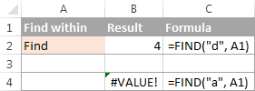
For example, the formula =FIND("d", "find") returns 4 because "d" is the 4th letter in the word "find". The formula =FIND("a", "find") returns an error because there is no "a" in "find".
Excel FIND function - things to remember!
To correctly use a FIND formula in Excel, keep in mind the following simple facts:
- The FIND function is case sensitive. If you are looking for a case-insensitive match, use the SEARCH function.
- The FIND function in Excel does not allow using wildcard characters.
- If the find_text argument contains several characters, the FIND function returns the position of the first character. For example, the formula FIND("ap","happy") returns 2 because "a" in the 2nd letter in the word "happy".
- If within_text contains several occurrences of find_text, the first occurrence is returned. For example, FIND("l", "hello") returns 3, which is the position of the first "l" character in the word "hello".
- If find_text is an empty string "", the Excel FIND formula returns the first character in the search string.
- The Excel FIND function returns the #VALUE! error if any of the following occurs:
- Find_text does not exist in within_text.
- Start_num contains more characters than within_text.
- Start_num is 0 (zero) or a negative number.
Excel SEARCH function
The SEARCH function in Excel is very similar to FIND in that it also returns the location of a substring in a text string. Is syntax and arguments are akin to those of FIND:
Unlike FIND, the SEARCH function is case-insensitive and it allows using the wildcard characters, as demonstrated in the following example.
And here's a couple of basic Excel SEARCH formulas:
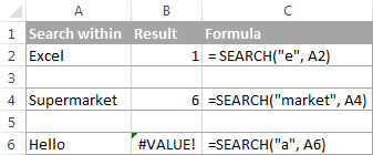
=SEARCH("market", "supermarket") returns 6 because the substring "market" begins at the 6th character of the word "supermarket".
=SEARCH("e", "Excel") returns 1 because "e" is the first character in the word "Excel", ignoring the case.
Like FIND, Excel's SEARCH function returns the #VALUE! error if:
- The value of the find_text argument is not found.
- The start_num argument is greater than the length of within_text.
- Start_num is equal to or less than zero.
Further on in this tutorial, you will find a few more meaningful formula examples that demonstrate how to use SEARCH function in Excel worksheets.
Excel FIND vs. Excel SEARCH
As already mentioned, the FIND and SEARCH functions in Excel are very much alike in terms of syntax and uses. However, they do have a couple of differences.
1. Case-sensitive FIND vs. case-insensitive SEARCH
The most essential difference between the Excel SEARCH and FIND functions is that SEARCH is case-insensitive, while FIND is case-sensitive.
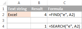
For example, SEARCH("e", "Excel") returns 1 because it ignores the case of "E", while FIND("e", "Excel") returns 4 because it minds the case.
2. Search with wildcard characters
Unlike FIND, the Excel SEARCH function accepts wildcard characters in the find_text argument:
- A question mark (?) matches one character, and
- An asterisk (*) matches any series of characters.
To see how it works on real data, consider the following example:
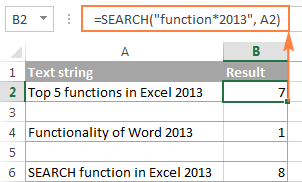
As you see in the screenshot above, the formula SEARCH("function*2013", A2) returns the position of the first character ("f") in the substring if the text string referred to in the within_text argument contains both "function" and "2013", no matter how many other characters there are in between.
Tip. To find an actual question mark (?) or asterisk (*), type a tilde (~) before the corresponding character.
Excel FIND and SEARCH formula examples
In practice, the Excel FIND and SEARCH functions are rarely used on their own. Typically, you would utilize them in combination with other functions such as MID, LEFT or RIGHT, and the following formula examples demonstrate some real-life uses.
Example 1. Find a string preceding or following a given character
This example shows how you can find and extract all characters in a text string to the left or to the right of a specific character. To make things easier to understand, consider the following example.
Supposing you have a column of names (column A) and you want to pull the First name and Last name into separate columns.
To get the first name, you can use FIND (or SEARCH) in conjunction with the LEFT function:
=LEFT(A2, FIND(" ", A2)-1)
or
=LEFT(A2, SEARCH(" ", A2)-1)
As you probably know, the Excel LEFT function returns the specified number of left-most characters in a string. And you use the FIND function to determine the position of a space (" ") to let the LEFT function know how many characters to extract. At that, you subtract 1 from the space's position because you don't want the returned value to include the space.
To extract the last name, use the combination of the RIGHT, FIND / SEARCH and LEN functions. The LEN function is needed to get the total number of characters in the string, from which you subtract the position of the space:
=RIGHT(A2,LEN(A2)-FIND(" ",A2))
or
=RIGHT(A2,LEN(A2)-SEARCH(" ",A2))
The following screenshot demonstrates the result:
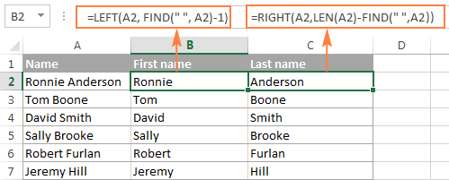
For more complex scenarios, such as extracting a middle name or splitting names with suffixes, please see How to split cells in Excel using formulas.
Example 2. Find Nth occurrence of a given character in a text string
Supposing you have some text strings in column A, say a list of SKUs, and you want to find the position of the 2nd dash in a string. The following formula works a treat:
=FIND("-", A2, FIND("-",A2)+1)
The first two arguments are easy to interpret: locate a dash ("-") in cell A2. In the third argument (start_num), you embed another FIND function that tells Excel to start searching beginning with the character that comes right after the first occurrence of dash (FIND("-",A2)+1).
To return the position of the 3rd occurrence, you embed the above formula in the start_num argument of another FIND function and add 2 to the returned value:
=FIND("-",A2, FIND("-", A2, FIND("-",A2)+1) +2)

Another and probably a simpler way of finding the Nth occurrence of a given character is using the Excel FIND function in combination with CHAR and SUBSTITUTE:
=FIND(CHAR(1),SUBSTITUTE(A2,"-",CHAR(1),3))
Where "-" is the character in question and "3" is the Nth occurrence you want to find.
In the above formula, the SUBSTITUTE function replaces the 3rd occurrence of dash ("-") with CHAR(1), which is the unprintable "Start of Heading" character in the ASCII system. Instead of CHAR(1) you can use any other unprintable character from 1 to 31. And then, the FIND function returns the position of that character in the text string. So, the general formula is as follows:
At first sight, it may seem that the above formulas have little practical value, but the next example will show how useful they are in solving real tasks.
Note. Please remember that the Excel FIND function is case-sensitive. In our example, this makes no difference, but if you are working with letters and you want a case-insensitive match, use the SEARCH function instead of FIND.
Example 3. Extract N characters following a certain character
To locate a substring of a given length within any text string, use Excel FIND or Excel SEARCH in combination with the MID function. The following example demonstrates how you can use such formulas in practice.
In our list of SKUs, supposing you want to find the first 3 characters following the first dash and pull them in another column.
If the group of characters preceding the first dash always contains the same number of items (e.g. 2 chars) this would be a trivial task. You could use the MID function to return 3 characters from a string, starting at position 4 (skipping the first 2 characters and a dash):
=MID(A2, 4, 3)
Translated into English, the formula says: "Look in cell A2, begin extracting from character 4, and return 3 characters".
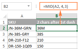
However, in real-life worksheets, the substring you need to extract could start anywhere within the text string. In our example, you may not know how many characters precede the first dash. To cope with this challenge, use the FIND function to determine the starting point of the substring that you want to retrieve.
The FIND formula to return the position of the 1st dash is as follows:
=FIND("-",A2)
Because you want to start with the character that follows the dash, add 1 to the returned value and embed the above function in the second argument (start_num) of the MID function:
=MID(A2, FIND("-",A2)+1, 3)
In this scenario, the Excel SEARCH function works equally well:
=MID(A2, SEARCH("-",A2)+1, 3)
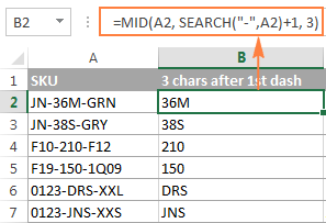
It's great, but what if the group of chars following the first dash contains a different number of characters? Hmm... this might be a problem:
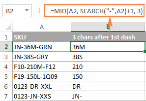
As you see in the above screenshot, the formula works perfectly for rows 1 and 2. In rows 4 and 5, the second group contains 4 characters, but only the first 3 chars are returned. In rows 6 and 7, there are only 2 characters in the second group, and therefore our Excel Search formula returns a dash following them.
If you wanted to return all chars between the 1st and 2nd occurrences of a certain character (dash in this example), how would you proceed? Here is the answer:
=MID(A2, FIND("-",A2)+1, FIND("-", A2, FIND("-",A2)+1) - FIND("-",A2)-1)
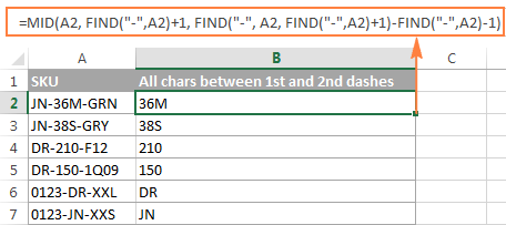
For better understanding of this MID formula, let's examine its arguments one by one:
- 1st argument (text). It's the text string containing the characters you want to extract, cell A2 in this example.
- 2nd argument (start_position). Specifies the position of the first character you want to extract. You use the FIND function to locate the first dash in the string and add 1 to that value because you want to start with the character that follows the dash: FIND("-",A2)+1.
- 3rd argument (num_chars). Specifies the number of characters you want to return. In our formula, this is the trickiest part. You use two FIND (or SEARCH) functions, one determines the position of the first dash: FIND("-",A2). And the other returns the position of the second dash: FIND("-", A2, FIND("-",A2)+1). Then you subtract the former from the latter, and then subtract 1 because you don't want to include either dash. As the result, you will get the number of characters between the 1st and 2nd dashes, which is exactly what we are looking for. So, you feed that value to the num_chars argument of the MID function.
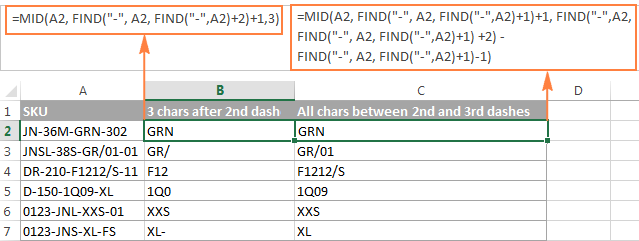
In a similar fashion, you can return 3 characters after the 2nd dash:
=MID(A2, FIND("-",A2, FIND("-", A2, FIND("-",A2)+1) +2), 3)
Or, extract all the characters between the 2nd and 3rd dashes:
=MID(A2, FIND("-", A2, FIND("-",A2)+1)+1, FIND("-",A2, FIND("-", A2, FIND("-",A2)+1) +2) - FIND("-", A2, FIND("-",A2)+1)-1)
Example 4. Find text between parentheses
Supposing you have some long text string in column A and you want to find and extract only the text enclosed in (parentheses).
To do this, you would need the MID function to return the desired number of characters from a string, and either Excel FIND or SEARCH function to determine where to start and how many characters to extract.
=MID(A2,SEARCH("(",A2)+1, SEARCH(")",A2)-SEARCH("(",A2)-1)
The logic of this formula is similar to the ones we discussed in the previous example. And again, the most complex part is the last argument that tells the formula how many characters to return. That pretty long expression in the num_chars argument does the following:
- First, you find the position of the closing parenthesis:
SEARCH(")",A2) - After that you locate the position of the opening parenthesis:
SEARCH("(",A2) - And then, you calculate the difference between the positions of the closing and opening parentheses and subtract 1 from that number, because you don't want either parenthesis in the result:
SEARCH(")",A2)-SEARCH("(",A2))-1
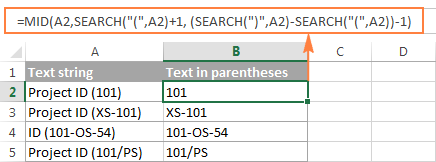
Naturally, nothing prevents you from using the Excel FIND function instead of SEARCH, because case-sensitivity or case-insensitivity makes no difference in this example.
Hopefully, this tutorial has shed some light on how to use SEARCH and FIND functions in Excel. In the next tutorial, we are going to closely examine the REPLACE function, so please stay tuned. Thank you for reading!
 by
by
423 comments
I want to find continues absent greater than 4 days like below
Amit AAAAAPPPPPPA Yes
Arun PAPPAPPPAPA NO
HI All,
look for guidance for I want find 1st character what the formula will be if my column got 2 criteria which is I want only show help what my formula will be?
1. help_request 123/123
2. help request 123/123
How to find Word'd position in string in Cell in Excel?
Example:
India, UK, USA, RSA (in A1)
UK (in B1)
Expected result in A2 2.
Where 2 is the position of word in A1. Like if RSA in B1 the answer should 4.
Hi Guys, my questions is straight forward:)
I have a column that has lots of sets of numbers but i want to extract only numbers that starts with 7 from left.
Thanks
Abdel
Filter with 7*
Dear, I am looking for the solution of occurrence of a repeated characters in a cell. I have data of contact numbers, like 01150000011, 01171222229, 01129999917 etc. I want to identify cells that have 5 or more than 5 consecutive numbers in phone number ( like 0 five times in first phone, 2 five times in 2nd phone and 9 six times in 3rd phone).
Hi,
This was to solve on the 60,000 data ,
Thanks & regards
Hi sir,
My name Niru,
My query is latest 10 days sales
Use Excel formulas.
Pass
Fail
Fail
Fail
Fail
I need "Pass" text separate from above list
Hi and thank you for the article.
Has anyone a suggestion on how to use a whole named range as the Search or Find Value?
Best, Phil
I currently have a formula that returns the last letter of T using this function:
=RIGHT(E2,LEN(E2)-SEARCH("-",E2)-4)
I then filter the data from there.......
I would like to search for multiple characters such as P, O , T.
Is there a function I can use to search for a set of letters without using advance filters?
Do you recommend just using advance filtering, if so what do I put into the criteria to find the numbers with Multiple characters.
B003-0144T
B003-0144P
B003-0144P
B003-0144P
B003-0144O
B003-0144O
B003-0144O
B003-0144E
B003-0144A
Thanks,
Willie
I currently have a formula that returns the last letter of T using this function:
=RIGHT(E2,LEN(E2)-SEARCH("-",E2)-4)
TB003-0144T
i got to say, your explanations provided me with a better understanding of the formula i was looking for. incase someone else is losing head over the same, below is a formula for returning text begining with "P" but ending before either " " or "-" =IF((SEARCH("-",C2))>(SEARCH(" ",C2,5)),MID(C2,SEARCH("P",C2),SEARCH(" ",C2,5)-SEARCH("p",C2)),MID(C2,SEARCH("P",C2),SEARCH("-",C2)-SEARCH("p",C2)))
Hi,
In the above example 3 "Extract N characters following a certain character", i see there is 3rd argument formulae, similar to that i have (4th and last argument) and (4th, 5th and last argument).
Ex 1: 123-345-456-78-46
Ex 2: 234-793-42-856-674-123
Ex 3: 123-345-456-789
i have numerous recrods/rows. i would like to split after "-" into each cell. I have tried to split using text to columns it worked out. But i would like to use the formulaes similar to example 3.
Can anyone help me to split the data, please.
Hello,
I have a excel sheet of attendance, For Example Employee Name:- Ajay Kumar Time :-09:06 J.p Site
And i want to create a new excel sheet which link with our attendance sheet . for example whenever Ajay kumar present on site So our new sheet will automatically appear in the present. What would the Formula be for this? Thank you.
Present Attendance Sheet
1. Ajay Kumar 09:06(J.P SITE)
New Attendance Sheet
1. Ajay Kumar (P) Show only present
I am trying to copy just the characters between the 2nd space and the 4th space. For instance, for the following cells, I want only "Lebron James" and Giannis Antetekounmpo" and Nikola Jokic". What would the formula be for this? Thank you.
L. James LeBron James SF/PF
G. Antetokounmpo Giannis Antetokounmpo SF/PF
N. Jokic Nikola Jokic C
Hello!
I would like to convert a string "John Watson Dalton" to "jwdalton". Can you help me?
Question? What formula could I use to search for a number value in a cell and give me the text description in the cell next to it
Lets say
A1= 8810 B2= Clerical
How do I create a formula to search for the number 8810 and bring up the Clerical description?
Amber:
I think you should try an approach that uses VLOOKUP.
The description and examples are here on AbleBits at:
https://www.ablebits.com/office-addins-blog/excel-vlookup-tutorial/
I have a full column of text with alphabetic as well numeric data, E.g 428538, 42H11, 225FL560, so what i want to do is if the text doesn't contain any Alphabet then I will take the last 2 numeric values as my req. data, but if the text contains alphabet then the letters needed are all letters before that as for 42H11=42, and for 225FL560=225, but also if the number before the alphabet are having more than 2 digits then the data needed is in the form of /10 so, e.g I will be needing output from 225FL560 as 22.5 and from 42H11 as 42, kindly help me..... thanks in avance...
There is a sentences in cell so how can v find number value in that sentence
Example:- i want to buy apple fruits of cost $50 per piece so I want retrieve only $50 from cell by using formulae
Mukesh:
Why not use the Text-to-Columns tool and set the 32 GB into its own column?
Hi
My Name is Mukesh Singh
Sir I have a query
Apple iPhone 6 32 GB Gold
I want "32 GB" in a separate cell using formula
Please help me to solve
Hi there,
I'm trying to fill in some missing data in my excel sheet. The method I am using is substitution where I have 6 columns. For example:
(Day) (Hour) (Wind direction) (wind speed) (stability) (rain in inches)
If I am missing the wind direction and wind speed I will look 2 weeks prior or after the missing data point for the same hour and stability and substitute those values in for the missing values. I used vlookup before and it would substitute from the top of the column or bottom but never the values closest from the missing data. My question is, is there a better method than the vlookup, would the find or search functions work? Or is there a method for vlookup to start from the missing data point and work away rather than starting from the top or bottom of the 2 week gap?
In my target string, the substring i want to extract is of the form Mxx - the letter M followed by a two digit number. THe target string will only have one occurrence of such a substring. The position of it though, is not fixed. For example:
F_8_M01_MASTER_MARKS_V15 - I am looking for M01.
F_8_M17_PTLY_XTV_V6 - I want to extract M17.
KB1F_MESURE_M34_FIN_V01.2 - I want to extract M34
How can I do that?
DesperatelyNeedHelp:
Here's a formula that will search a string and return the value you enter into a cell.
You can do it two ways I'll show you both and you can decide which one works best for you.
OK, you can enter the search value directly into the formula like this;
Where F_8_M17_PTLY_XTV_V6 is in B13 enter this formula into an empty cell.
=IF(B13="","",IF(ISNUMBER(SEARCH("M17",B13)),"M17"))
Alternatively you can enter the search value into a cell and reference that cell in the formula like this:
=IF(B13="","",IF(ISNUMBER(SEARCH(D2,B13)),D2))
Where F_8_M17_PTLY_XTV_V6 is in B13 and you enter M17 into D2 this will return M17 into the cell where this formula is.
i want to find a text 'P' in a string which is then followed by 3 numbers. The 3 numbers can be anything.
If I understand your question this formula should work.
Where "P123" is in A44 enter this in an empty cell:
=MID(A44,FIND("P",A44),1)
col A contains some set of strings, Col B contains some Sub-strings , and the corresponding coloumn C should return values of string which contains the particular substring.
what formula can be used to pull out the string which contains this particular sub-string
Col A Col B col C
ABCD-alpha rain rainrain-rhyme
1234-num abc ABCD-alpha
rainrain-rhyme numb 1234-num
Lavanya:
Here's a formula that works if there are no duplicates,
=IFERROR(INDEX($A$1:$A$5,MATCH(TRUE,INDEX(ISNUMBER(SEARCH(B1,$A$1:$A$5)),,),0)),"No Match")
Just copy this down the C column and it will return the string from the A column that contains the sub-string found in the B column.
You can expand the $A$1:$A$5 range. The B1 will change as you copy it down the C column.
FYI, the "numb" in your sample will return the "No Match".
Absolutely the best post that I found on this subject!
This is comprehensive and detailled, yet very clear and easy to understand. The choice of examples just adds to that.
Thank you very much, this post was truly helpful.
Kindest regards
Pieter
Hi,
I have a problem in excel for find and pest,
The problem is "in a excel one page i have some numbers(123456), same page same number included in some words(abcd123456), so i can find out based on any formula please let me know, i am waiting.
Hello,
I am trying to figure out how to do the following:
Count the number of cells which have the character + within the word.
Each of over 60 columns will have a different word.
E.g. BOB+CAT, DOG+BIRD, CAN+, etc.
Count Number of Cells That Contain Specific Character
=COUNTIF(A23:A29,"*+*")
Where A23:A29 is the range of cells you want to count the number of times the “+” character is in the text.
hello madam..
good morning..
we want some help from you..
we just want to confirm why we use find and replace formula...
we use find and replace formula from home menu or by pressing(ctrl+f)..
Hi,
To get around the #VALUE problem, you can use the ISERROR() function. For example, if you have a cell, A1, and you want to check the position of the letter p, you can use:
=IF(ISERROR(FIND("p",A1)),0,FIND("p",A1))
If the letter p is present, this will report the position. If not, it will report 0.
The first section, ISERROR(FIND("p",A1)), determines if p is present. If not, the IF returns 0. If there is no error, the IF then looks again for p and reports its actual position.
i have several file names extracted to excel with the "009-?-????" string as part of the filename. i need to extract this string from the remaining file name. the question marks are wild card.
Hi,
I require to find out the number of spaces before any text in a cell from starting. For Example:
" A56020 - Depr - buildings"
We have to find out the length of blanks before any first text. Here blanks are 20 before first text (here first text is A, it is different in different cells).
Any help is of great help.
Thanks,
DG
What if...
A1 UK-USA and B1 1-0
A2 USA-UK B2 0-1
A3 USA-UK B3 4-3
A4 UK-USA B4 2-1
A5 UK-USA etc.
A6 USA-UK
etc.
How to return with a function ALL UK results in left-right order in C1... like
C1 is 1-0
C2 is 1-0
C3 is 3-4
C4 is 2-1
etc.
Thanks...
Svetlana, I can't thank you enough for sharing this knowledge with us!
These functions are super useful when used appropriately, and you've given an excellent explanation of how and where to use these. Rock on.
Hi Svetlana! I think I posted this question in the wrong topic, so posting again here with more details.
I need to extract a string between two other strings (a word and a character) within a cell, but those other strings may repeat inside the cell at different intervals.
For example - a scanning tool conducts several tests and returns all of the results within a cell, but we only want information on the failures
multi-line cell example:
Test: Endpoint
Result: Pass
Details: Endpoint Connected
*****
Test: Resolution
Result: Fail
Details: Unable to resolve FQDN
*****
Test: Port
Result: Fail
Details: Port 1234 does not respond
We initially tried to re-organize the output using text to columns but it seems to be thrown off by the carriage returns inside the cell and ideally, we want to wan).
So we're left with searching for some combination of MID, SEARCH, and maybe LEN functions? but it's proving very difficult. It's easy to find the first instance of "Failed", but to then find the stopping point which has to be the very next "^" char after that instance of "Failed", while also then being able to repeat the extraction for any other Failed tests inside the same cell.
Hi Svetlana, I am trying to use Find or Search function for multiple conditions, how can I use this?
I have a table where I want to extract the first name from full name but the values are not consistent. I am getting different values in different cells for example:
Full Name:
Derek Gorgi
Jonathan, Kelly
Now I am trying to extract the first name before " " and/or before "," then how can I use Find or Search function to get the First Name without Space or comma
To get the First value where I was getting only space, I was using the following formula as shown below but not sure how can I inculcate multiple search criteria as mentioned above.
=LEFT(A2, FIND(" ",A2,1)-1)
Please help.
Thanks
Sandeep
hello sandeep sir..
according to me..
no need to apply (-1) in the formula =LEFT(A2, FIND(" ",A2,1)-1)
formula is:
=LEFT(A2,FIND(" ",A2,1))
SEARCH is not case sensitive. Please correct.
Hello,
The article says that FIND is case-sensitive and SEARCH is case-insensitive. That's exactly what you say :)
Can someone clarify my surmise: EXCEL does not support searching of text with wild card that involve MULTIPLE Criteria Using the FILTER menu. Say,
Finding all the records in which the Name filed either BEGINS with John OR ends with Higgins? I tried and and not get the desired results; it does not report error but gives only those records satisfying first criterion.
Hi,
I would like to ask on how to create a formula in searching one word to another tab. Like for example, i need to get the word apple in other tab but the word from that tab is apple pie, the formula i need is to get all with the word apple.
Thanks in advance
=LEFT(A1,FIND("*",A1))
Ma'am Lets say i have (3242*4643) and i have to extract from ( to * then what would i have to do?
Hi,
I have a problem in excel for find and pest,
The problem is "in a excel one page i have some numbers(123456), same page same number included in some words(abcd123456), so i can find out based on any formula please let me know, i am waiting.
Wonderful.
Thank you
Hello. This page is great. Thank you for sharing. Question, Your number 4, Find text between parentheses.... How do I apply this to multiple to an excel sheet that has many multiple lines of data? Each Line will have information in parentheses and we would like to pull the information within the parentheses from each line? Would I need to apply the formula =MID(D1,SEARCH("(",D1),SEARCH(")",D1)-SEARCH("(",D1)+1) to each line of data or is there an easy way to drag and select multiple line? (I know this formula includes the parentheses, which is what we want). Thanks!
Hello,
I'm afraid there's no easy way to solve your task with a formula. Using a VBA macro would be the best option here.
However, since we do not cover the programming area (VBA-related questions), I can advice you to try and look for the solution in VBA sections on mrexcel.com or excelforum.com.
Sorry I can't assist you better.
Hi,
Great set of examples on how to go about finding stuff in excel cells. I have a question though which i haven't found in your examples (or overlooked). I get a data dump with a json string in a cell. In json there is a lot of use of the " character. I can't seem to figure out how to look for a " in a cell.
Placing it in '"' (single quotes surrounding the ") didn't help either. Is this at all possible and if so how?
Hi Remi,
Please try to use one of the following formulas:
1. =FIND("""",A1)
2. =FIND(CHAR(34),A1)
Hope this will work for you.
In one tab ('Orchard details')of a spreadsheet I have a list of our 14 orchards and their respective varieties in each orchard. Some orchards have more than one variety. Some orchards have the same variety as other orchards. One field in the list is fallow at present. This list is in cells AA6:AA27. In another tab ('Orchard varieties'), I want to create just a list of the varieties that we grow taken from the 'Orchard details' list, reporting the (orchard varieties' tab in cells B93:B105. As we grub old orchards and plant new ones we may change the variety so the 'Orchard varieties' list would need to change as we replant our orchardsand record them in the 'Orchard details' list. Thank you.
Hi,
I have a column with multi-word text strings, I'd like to look in that text and for any cell in the column that contains one of three (e.g.) words, I'd like to return "X", else "Y".
For example, if the text contains 'green', 'blue' or 'purple' I'd like the result to be 'cool' else 'warm'
COL A COL B (result)
light pink warm
forest green cool
ocean blue cool
burnt orange warm
thanks,
sorry...didn't know spaces wouldn't be retained.
Col A | Col B(result)
light pink | warm
forest green | cool
ocean blue | cool
burnt orange | warm
Nevermind...unless there is an easier solution.
This works:
=IFERROR(IF(FIND("GREEN",$BJ34),"Cool","Warm"),IFERROR(IF(FIND("BLUE",$BJ34),"Cool","Warm"),IFERROR(IF(FIND("PURPLE",$BJ34),"Cool","Warm"),"Warm")))
I suppose 'Search' instead of 'Find' is optional if there is concern about being case-sensitive.
Hi,
I'm using the below formula to extract data (equipment number) with a hyphen. For example, cell contains:
V-1770A BLAST/PAINT EXTERNAL SURFACE (#17337C)
the formula:
=TRIM(MID(SUBSTITUTE(E3080," ",REPT(" ",99)),MAX(1,FIND("V-",SUBSTITUTE(E3080," ",REPT(" ",99)))-50),99))
returns the results:
V-1770A
The formula works great, but I have to change the FIND find_text parameter for each line.
Examples of various data lines:
I-1602 A/B "DRYER" DEMO SCAFFOLD # 2080 (#17324A)
E-1403 "IN/OUTLET VALVE " DEMO SCAFFOLD #2076 (#17324A)
C-1407 "INSPECTION WINDOWS" REPLACE METAL/SEALANT (#17324B)
T-1311C "ROOF TOP NOZZLES" CLEAN/PAINT (#17324C)
V-1770A BLAST/PAINT EXTERNAL SURFACE (#17337C)
No matter where the information is on the line the formula works, but I do not want to have to edit the formula each time the equipment letter changes.
I've tried using a Define Name table in the find_text parameter, but that does not work. Returns #VALUE.
Any suggestions or help would be greatly appreciated.
6601280012088
How do I extract the 7th number. =mid(C7,7,1)
if greater/equal to 7 - indicate "Male" otherwise "Female"
Hi,
I am trying to find a formula to yield the word to the left of the first space at the right. For example in the first item below, I would want the formula to result in BRAZR. The reason I cant work from the left (or at least I cant seem to) is there is a different number of spaces to get to the word to the left of the last space on the right as you can see below with the other examples. Could you please help me out with this??
XXX 5C-15 HZ BRAZR 3-14-47-14
XXX KARR 13-28-65-3
XXX HZ LEDUC-WB 16-9-49-25
XXX HZ BANTRY 4-21-19-13
Much appreciated.