The IF function in Google Sheets is one of the easiest functions to learn, and while this holds true, it is also a very helpful one.
In this tutorial, I invite you to take a closer look at how Google Spreadsheet IF function works and what advantages you will get from using it.
What is the IF function in Google Sheets?
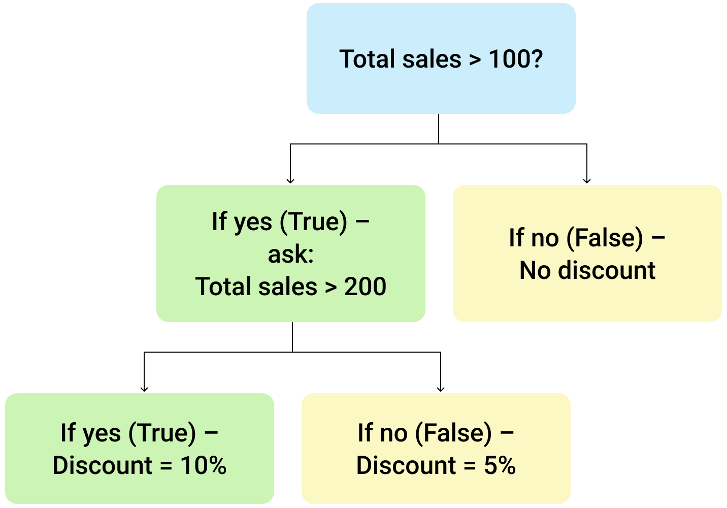
Whenever you use the IF function, you create a decision tree in which certain action follows under one condition, and if that condition is not met – another action follows.
For this purpose, the condition of the function must be in a format of the alternative question with only two possible answers: "yes" and "no".
This is what a decision tree may look like:
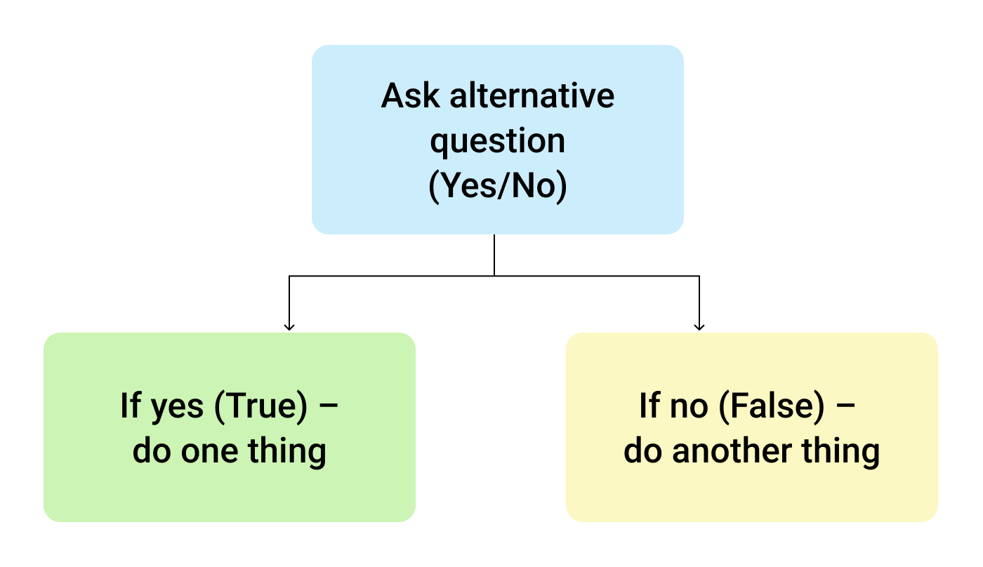
So, the IF function allows you to ask a question and indicate two alternative actions depending on the received answer. This question and the alternative actions are known as three arguments of the function.
IF function syntax in Google Sheets
The syntax for the IF function and its arguments are as follows:
- logical_expression – (required) a value or logical expression that is tested to see if it is TRUE or FALSE.
- value_if_true – (required) the operation that is carried out if the test is TRUE.
- value_if_false – (optional) the operation that is carried out if the test is FALSE.
Let's explore the arguments of our IF function in more detail.
The first argument represents a logical question. Google Sheets answers this question with either "yes" or "no", i.e. "true" or "false".
How to formulate the question properly, you may wonder? To do that, you can write a logical expression using such helpful symbols (or comparison operators) as "=", ">", "<", ">=", "<=", "<>". Let us try and ask such a question together.
Usage of the IF function
Let's assume that you are working in the company selling chocolate in several consumer regions with many clients.
This is what your sales data may look like in Google Sheets:
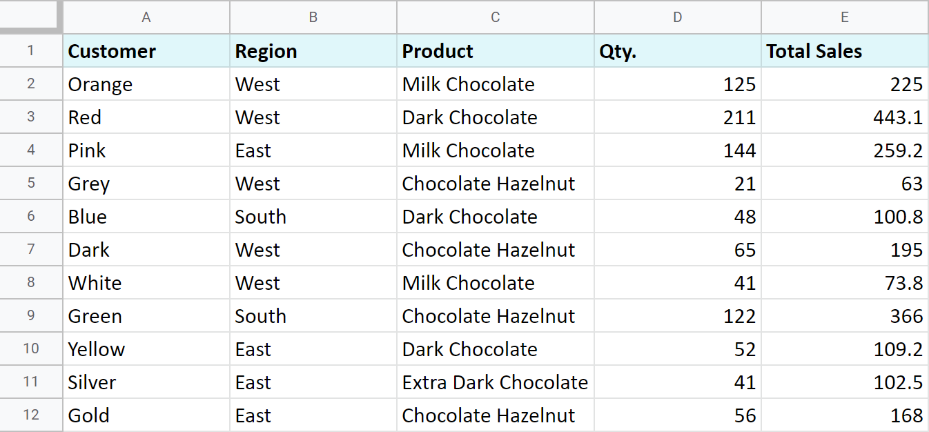
Imagine that you need to separate sales made in your local regions from those from abroad. To accomplish that, you should add another descriptive field for each sale – a country where the sales took place. Since there is a lot of data, you need this description field to be created automatically for each entry.
And this is when the IF function comes to play. Let's add the "Country" column to the data table. "West" region represents local sales (Our Country), while the rest are the sales from abroad (Rest of the World).
How to write out the function properly?
Place the cursor in F2 to make the cell active and type in the equality sign (=). Google Sheets will immediately understand that you are going to enter a formula. That's why right after you type the letter "i" it will prompt you to choose a function that begins with that same letter. And you should choose "IF".
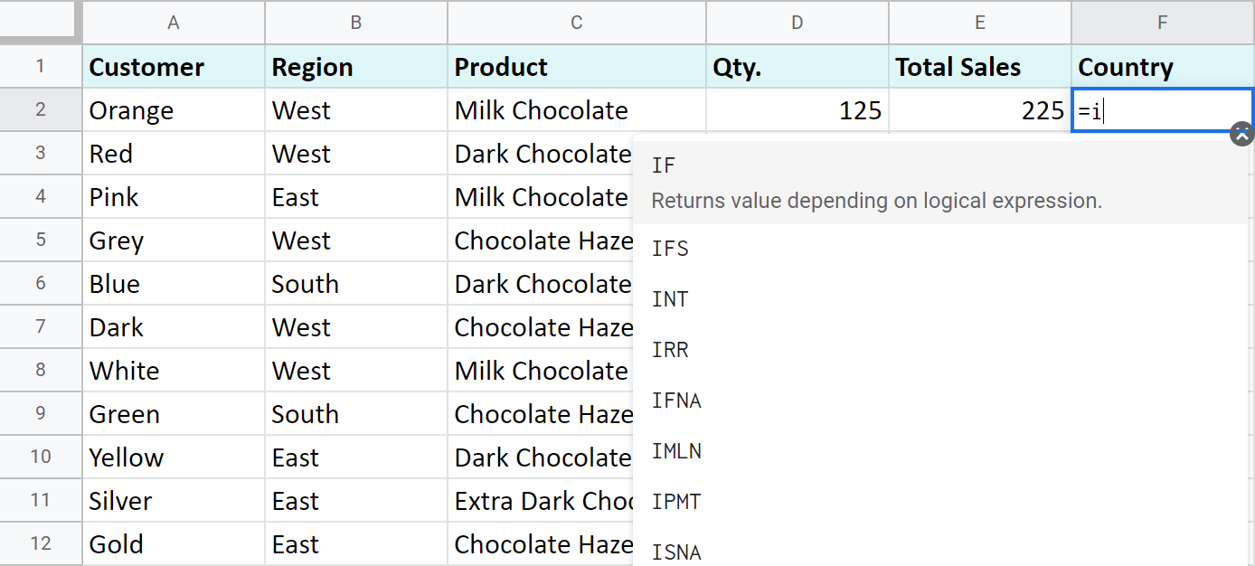
After that, all your actions will be accompanied by prompts as well.
For the first argument of the IF function, enter B2="West". As with the other Google Sheets functions, you don't need to enter the address of the cell manually – a mouse click is enough. Then enter comma (,) and specify the second argument.
The second argument is a value that F2 will return if the condition is met. In this case, it will be the text "Our Country".
And again, after the comma, write the value of the 3rd argument. F2 will return this value if the condition is not met: "Rest of the World". Do not forget to finish your formula entry by closing parenthesis ")" and pressing "Enter".
Your entire formula should look like this:
=IF(B2="West","Our Country","Rest of the World")
If everything is correct, F2 will return the text "Our Country":
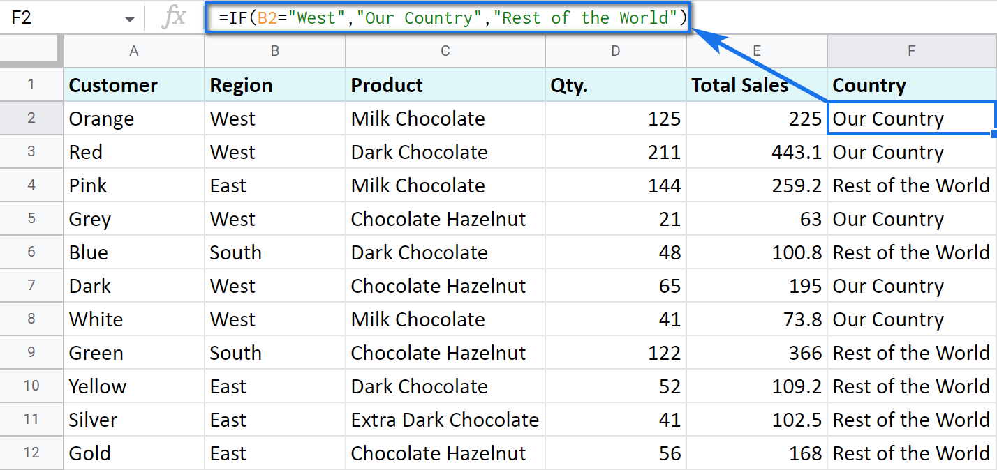
Now, all you have to do is to copy this function down column F.
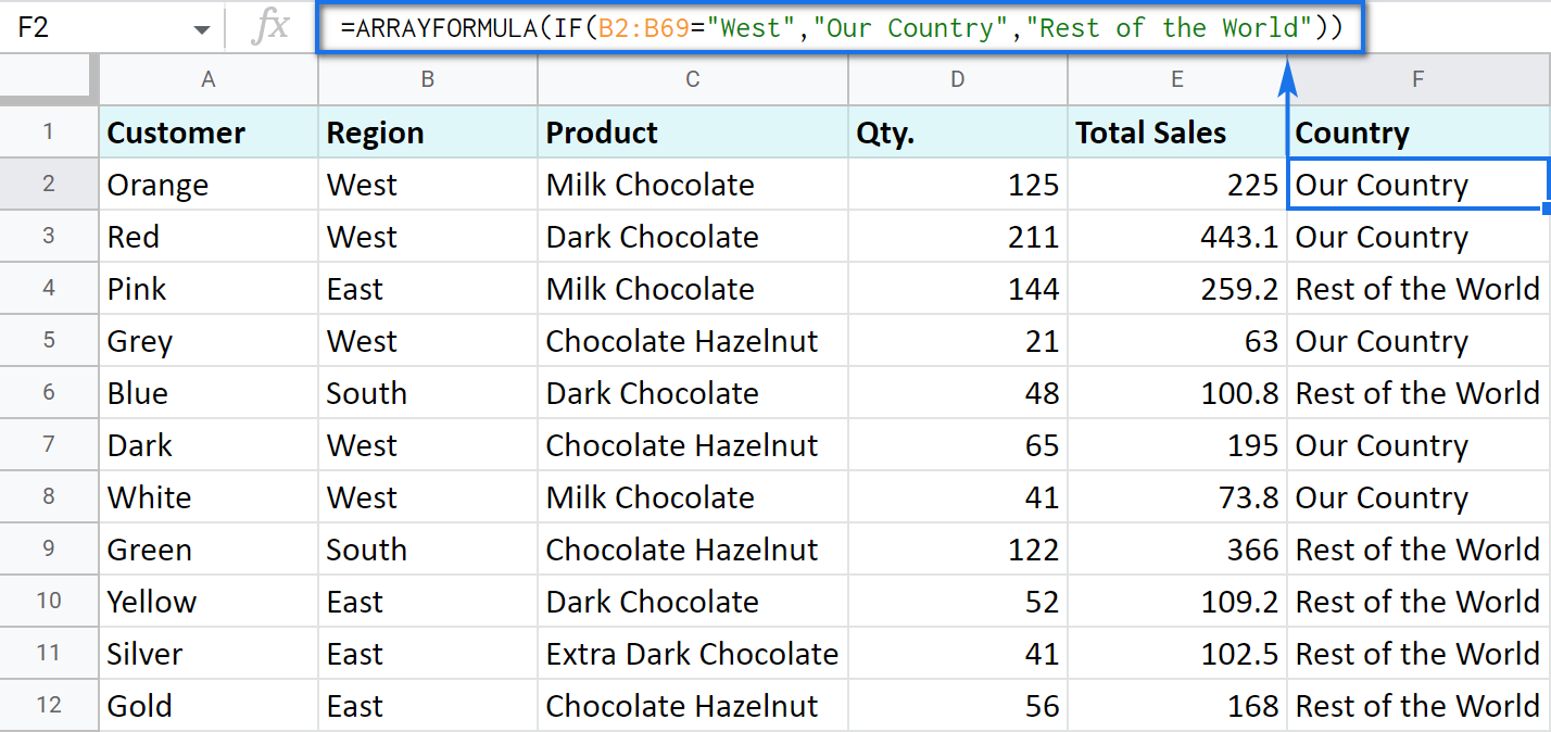
Tip. There's one way to process the entire column with one formula. The ARRAYFORMULA function will help you do that. Using it in the first cell of the column, you can test all cells below against the same condition, and return the corresponding result to each row at the same time:
=ARRAYFORMULA(IF(B2:B69="West","Our Country","Rest of the World"))
Let's examine the other ways of working with the IF function.
IF function and text values
The usage of the IF function with a text has already been illustrated in the example above.
Note. If the text is being used as the argument, then it must be enclosed in double-quotes.
IF function and numerical values
You can use numbers for the arguments just as you did with the text.
However, what is very important here is that the IF function makes it possible to not only fill cells with certain numbers based on the conditions met but also calculate.
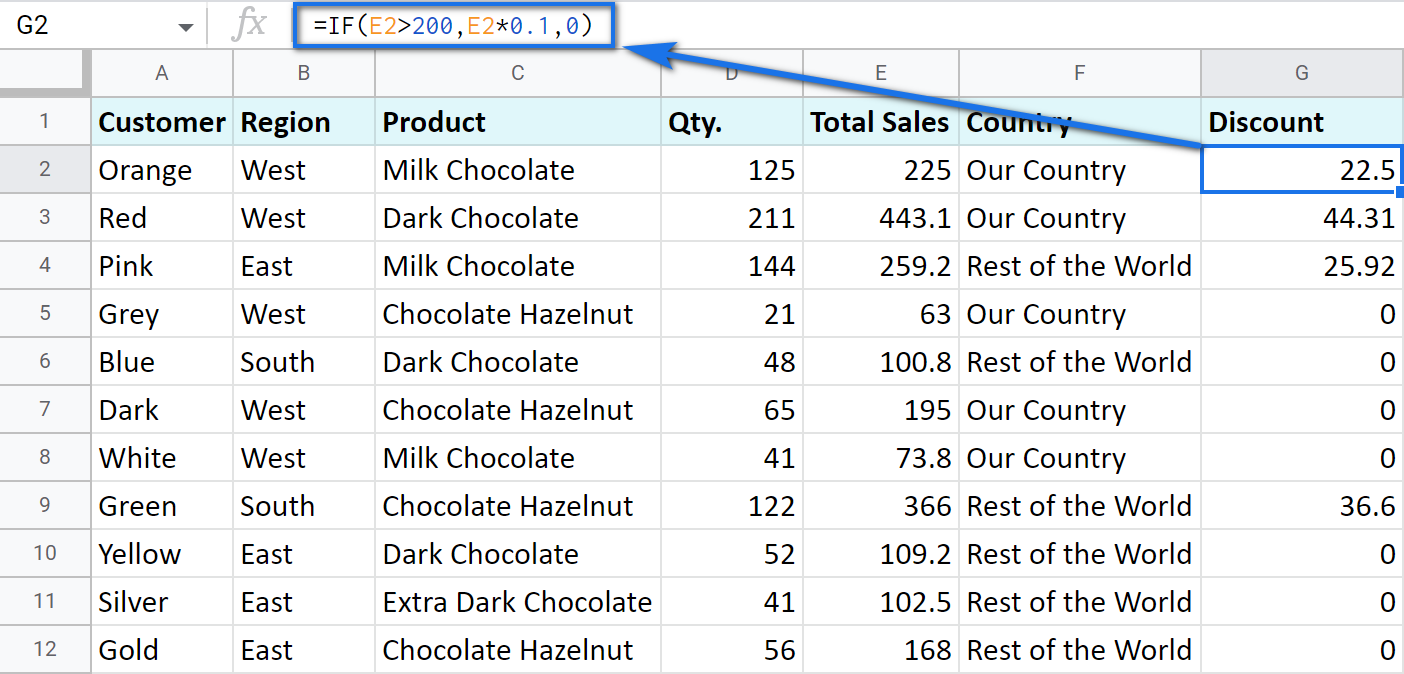
For example, let's say you offer your clients various discounts based on the total value of the purchase. If the total is more than 200, then the client gets a 10% discount.
For that, you need to use column G and name it "Discount". Then enter the IF function in G2, and the second argument will be represented by the formula that calculates the discount:
=IF(E2>200,E2*0.1,0)
IF blanks/non-blanks
There are cases when your result depends on whether the cell is empty or not. There are two ways to check that:
- Use the ISBLANK function.
For example, the following formula checks if cells in column E are empty. If so, no discount should be applied, otherwise, it's 5% off:
=IF(ISBLANK(E2)=TRUE,0,0.05)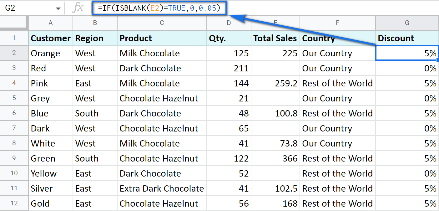
Note. If there's a zero-length string in a cell (returned by some formula), the ISBLANK function will result in FALSE.
Here is another formula to check if E2 is empty:
=IF(ISBLANK(E2)2<>FALSE,0,0.05)You can turn the formula the other way around and see if cells are not blank instead:
=IF(ISBLANK(E2)=FALSE,0.05,0=IF(ISBLANK(E2)<>TRUE,0.05,0) - Use standard comparison operators with a pair of double-quotes:
Note. This method considers zero-length strings (indicated by double-quotes) as empty cells.
=IF(E2="",0,0.05)– check if E2 is blank=IF(E2<>"",0,0.05)– check if E2 is not empty.Tip. In a similar manner, use double-quotes as an argument to return an empty cell by the formula:
=IF(E2>200,E2*0,"")
IF in combination with other functions
As you have already learned, the text, numbers, and formulas can act as the arguments of the IF function. However, other functions can play that role as well. Let's see how it works.
Google Sheets IF OR
Remember the first way you figured out the country where you sold chocolate? You checked if B2 contained "West".
However, you can build the logic the other way around: list all the possible regions that belong to the "Rest of the World" and check if at least one of them appears in the cell. The OR function in the first argument will help you do that:
- logical_expression1 – (required) the first logical value to check for.
- logical_expression2 – (optional) the next logical value to check for.
- and so on.
As you can see, you just enter as many logical expressions as you need to check and the function searches if one of them is true.
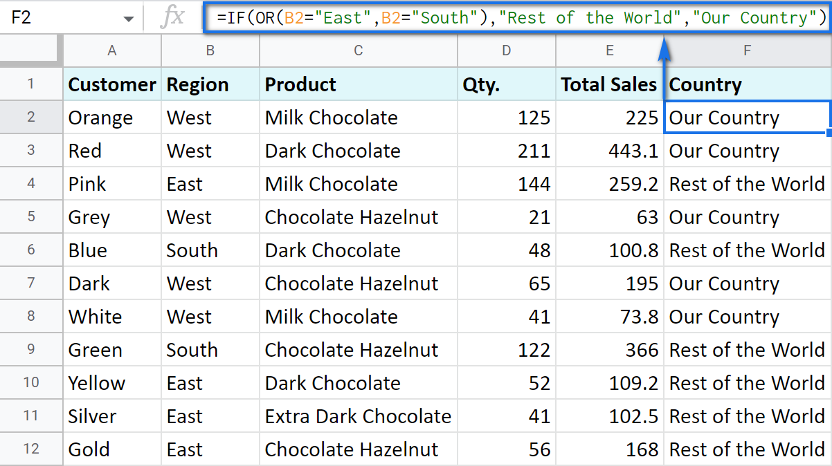
To apply this knowledge to the table with sales, mention all the regions that belong to the sales abroad, and the other sales will automatically become local:
=IF(OR(B2="East",B2="South"),"Rest of the World","Our Country")
Google Sheets IF AND
The AND function is just as simple. The only difference is that it checks if all listed logical expressions are true:
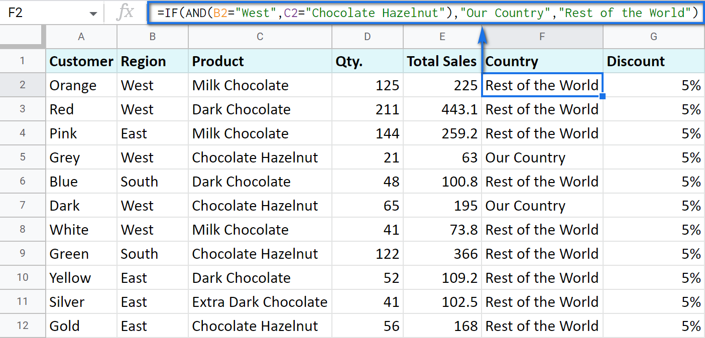
E.g. you need to narrow the search to your town and you know that it is currently buying only hazelnuts. So there are two conditions to consider: region – "West" and product – "Chocolate Hazelnut":
=IF(AND(B2="West",C2="Chocolate Hazelnut"),"Our Country","Rest of the World")
Nested IF formula vs. IFS function for Google Sheets
You can also use the IF function itself as an argument for the bigger IF function.
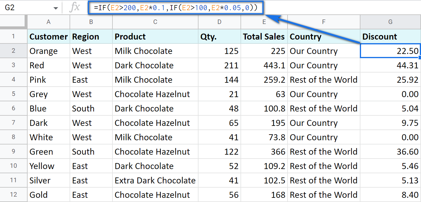
Let's assume that you have set stricter discount conditions for your clients. If the total purchase is more than 200 units, they get a 10% discount; if the total purchase is between 100 and 199, the discount is 5%. If the total purchase is lower than 100, there is no discount whatsoever.
The following formula shows how the function will look in the cell G2:
=IF(E2>200,E2*0.1,IF(E2>100,E2*0.05,0))
Note that it is another IF function that is used as the second argument. In such cases, the decision tree is as follows:
Let's make it even more fun and complicate the task. Imagine that you're offering the discounted price to the one region only - "East".
To do that correctly, add the logical expression "AND" to our function. The formula will then look the following way:
=IF(AND(B2="East",E2>200),E2*0.1,IF(AND(B2="East",E2>100),E2*0.05,0))
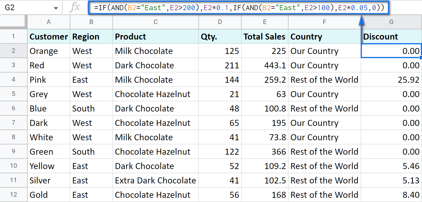
As you can see, the number of discounts has reduced greatly while their amount remains intact.
There's also an easier way to write the above thanks to the IFS function:
- condition1 – (required) is the logical expression you want to test.
- value1 – (required) is the value to return if the condition1 is true.
- and then you just list conditions with their values to return if they are true.
Here's how the above formula will look with IFS:
=IFS(AND(B2="East",E2>200),E2*0.1,AND(B2="East",E2>100),E2*0.05)
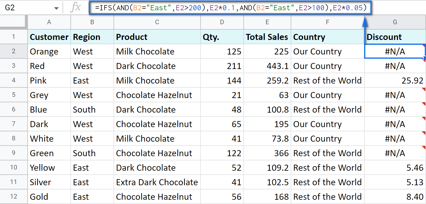
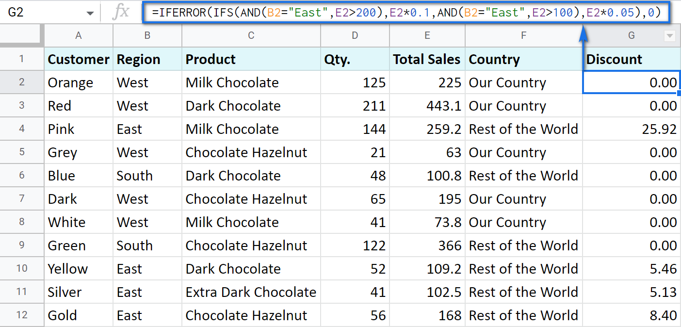
Tip. If there's no true condition, the formula will return the #N/A error. To avoid that, wrap your formula with IFERROR:
=IFERROR(IFS(AND(B2="East",E2>200),E2*0.1,AND(B2="East",E2>100),E2*0.05),0)
SWITCH as an alternative to multiple IFs
There's one more function you may want to consider instead of the nested IF: Google Sheets SWITCH.
It checks if your expression corresponds to a list of cases, one by one. When it does, the function returns a corresponding value.
- expression is any cell reference, or a range of cells, or even an actual math expression, or even a text that you'd like to equal to your cases (or test against the criteria). Required.
- case1 is your first criteria to check the expression against. Required.
- value1 is a record to return if the case1 criterion is the same as your expression. Required.
- case2, value2 repeat as many times as criteria you have to check and values to return. Optional.
- default is also completely optional. Use it to see a specific record if none of the cases is met. I'd recommend using it every time to avoid errors when your expression doesn't meet matches among all the cases.
Here are a couple of examples.
To test your cells against a text, use ranges as an expression:
=ARRAYFORMULA(SWITCH(B2:B69,"West","Our Country","Rest of the World"))
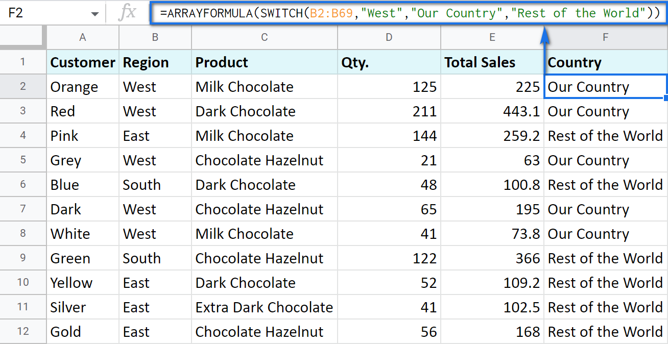
In this formula, SWITCH checks what record is in every cell in column B. If it's West, the formula says Our Country, otherwise, Rest of the World. ArrayFormula makes it possible to process the entire column at once.
To work with calculations, it's better to use a boolean expression:
=SWITCH(TRUE,$E2>200,$E2*0.1,AND($E2<200,$E2>100),$E2*0.05,0)
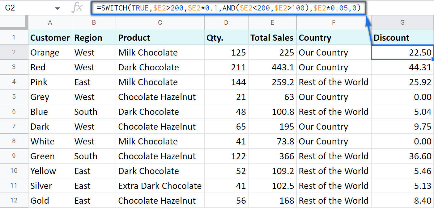
Here SWITCH checks if the result of the equation is TRUE or FALSE. When it's TRUE (like if E2 is really greater than 200), I get a corresponding result. If none of the cases in the list is TRUE (meaning they are FALSE), the formula simply returns 0.
Note. SWITCH doesn't know how to calculate the entire range at once, so no ARRAYFORMULA in this case.
IF statements based on a count
One of the questions we get asked a lot is how to create the IF formula that will return whatever you need if the column contains or doesn't contain a certain record.
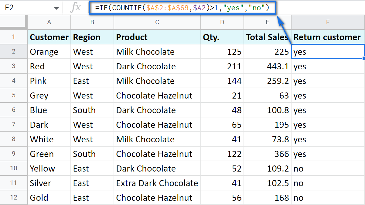
For example, check if a customer's name appears more than once in a list (column A) and put the corresponding word (yes/no) into a cell.
A solution is simpler than you may think. You need to introduce the COUNTIF function to your IF:
=IF(COUNTIF($A$2:$A$69,$A2)>1,"yes","no")
Make Google Sheets build IF formulas for you – IF Formula Builder add-on
If you're tired of keeping track of all those extra characters and proper syntax in formulas, there's another solution available.
IF Formula Builder add-on for Google Sheets offers a visual way of creating IF statements. The tool will handle syntax, extra functions and all required characters for you.
All you need to do is:
- fill blanks with your records one by one. No special treatment for dates, time, etc. Enter them as you always do and the add-on will recognize the data type.
- select required comparison operators from the suggested drop-down lists.
- if needed, add multiple logical expressions in a click: IF OR, IF AND, ELSE IF, THEN IF.
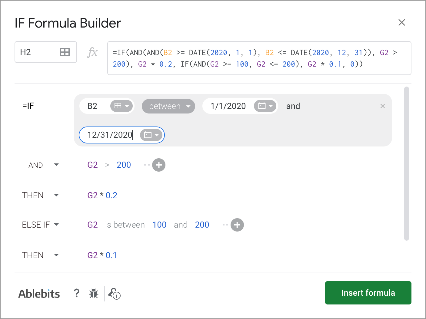
As you can see, each logical expression takes its own line. The same goes for true/false outcomes. This reduces the number of possible confusion over the formula drastically.
As you fill everything out, the formula for use will grow in the preview area at the top of the window. To its left, you can select a cell in your sheet where you'd like to have the formula.
When you're ready, paste the formula into the cell of interest by clicking the Insert formula button at the bottom.
Please visit the online tutorial for IF Formula Builder to see all options described in detail.
I hope that there's no room for any doubt now that the IF function, though a very simple one at first glance, opens the door to many options for data processing in Google Sheets. But if you still have questions, feel free to ask them in the comments section down below – we'll be happy to help!
 by
by
601 comments
Hi there thanks for the amazing article! it's helped a lot.
I currently am having an issuewith my if + vlookup statements.
My current string:
=if(B1=5,=VLOOKUP(I1,data!A:D,2),VLOOKUP(I1,data!A:D,3))
If B1=5 I want it to look up I1's data in Collumn 2
If B1=6 I want it to look up I1's data in Collumn 3
If B1=7 I want it to look up I1's data in Collumn 4
example
B1 I1 J1
5 10 =look at number 10 Collumn 6 and give that back
Hi Caleb,
If I'm getting your task clear, you should nest several IFs for multiple conditions like this:
=IF(B1=5,VLOOKUP(I1,data!A:D,2),IF(B1=6,VLOOKUP(I1,data!A:D,3),IF(B1=7,VLOOKUP(I1,data!A:D,4))))
I am trying to change the color based on a column with a dropdown to color a gantt. Any help would be great
=IF(F4 ='Ministry', SPARKLINE(if(OR(today()D4),{int(C4)-int($C$2),if(C4=D4,1,int(D4)-int(C4))},{int(C4)-int($C$2),today()-int(C4),1,int(D4)-today()}),{"charttype","bar";"color1","white";"Light Blue"}),
IF(F4 = 'Project',SPARKLINE(if(OR(today()D4),{int(C4)-int($C$2),if(C4=D4,1,int(D4)-int(C4))},{int(C4)-int($C$2),today()-int(C4),1,int(D4)-today()}), {"charttype","bar";"color1","white";"Light Blue"}),
IF(F4 = 'Cerner/AscTech',SPARKLINE(if(OR(today()D4),{int(C4)-int($C$2),
if(C4=D4,1,int(D4)-int(C4))},{int(C4)-int($C$2),today()-int(C4),1,int(D4)-today()}),{"charttype","bar";"color1","white";"Light Blue"}),)));"max",int($D$2)-int($C$2)}
Hello Anthony,
You may find this YouTube video tutorial useful: Creating a Gantt Chart in Google Sheets. The author starts introducing colors at 9:10.
I am trying to use an if statement based on a data validation "yes" or "no" If the answer is yes the result will be a hyperlink (in a label) which the user can click to. If the the data validation is blank then the result is blank. If the answer is "no" I wish to return a text response. I am getting the hyperlink by getting the link from a different area in the sheet.
Can anyone help as its driving me mad!
Hello Lloyd,
Supposing your data validation is in A2, the link is in B2, the formula you need can be as simple as this:
=IF(A2="yes",B2,IF(A2="no","your_text_response",""))
I'm looking for a formula for this
A B C
1 Red 50 Lunch
2 Black 72 Dinner
3 Blue 83 Lunch
4 Orange 17 Lunch
5 Green 23 Dinner
Totals
8 Lunch
9 Dinner
I want the SUM of Lunches that is in column B to show in B8 (150) and the SUM of Dinners that is in column B to show in B9 (95). How would I write out the formula? This is just an example of what I want to do, it's really for different bills (A) that are in different categories (C). The amount is in column B. I basically want the B's to add up by category below in row 8 and 9.
Hello Jeremy,
please refer to blog posts about SUMIF and SUMIFS to solve your task.
Hey,
I am trying to design a grade calculator for my students but I am stuck!
I have made a dropdown with YES or NO in one column for certain units of work, and I need the formula for if they put 'yes' in all boxes it needs to show distinction, if they put yes in some and no in others its a merit or pass (dependence on answers to yes and no's)
Anyone have any answers? I have been googling for a while!
Any help would be ace!
Hey Jacky,
I'm afraid your task is not clear. With those little details you provided, I can only suggest how to start the formula: =IF(COUNTIF(A2:A10,"Yes")=9,...), where A2:A10 is a supposed column with the answers.
What distinction should be seen and where if all answers are 'yes'? Also, "its a merit or pass (dependence on answers to yes and no’s)" please specify when it should be 'merit' or 'pass' exactly.
Disregard previous question.
Hello Joshua,
Just in case you found the solution with the IF function, I'd recommend looking into SUMIF or SUMIFS :)
Is there a way to write a function that keeps track of the sum of certain values in a column, if different column values meet a certain criteria into one cell.
I have a chart to keep track of certain expenses for my building business.
In one column it gives the "type of material" and then in another column it has the purchase amount. The type of materials change(ie: plumbing, framing, kitchen), so i need to get the sum of only certain values.
Materials Type Purchase Amount
Plumbing $20.00
Trim $10.00
Plumbing $20.00
Is there a way on one cell to find the sum of only the plumbing total?
Please disregard my previous email. A simple 'refresh' did the trick. Duh!
Hi, I am a teacher and I'm trying to create a spreadsheet to track whether or not my students' test grades meet certain criteria.
I have typed: =if(H7>=65,"yes","no)
But when I hit Enter, the entire, exact formula is what shows up in the cell (not the 'yes' or 'no').
Receiving a "VALUE" message when trying to add two if statements;
D1 cell input; =SUM(IF(A2="x",E15,0)+IF(A3="x",E16,0); D1 displays "#VALUE"
Cell References; E15=$40; E16=$20
When separating the if statements into separate cells, values appear:
D2 cell input; =IF(A2="x",E15,0); D2 Displays $40 value
D3 cell input; =IF(A3="x",E16,0); D3 Displays $20 value
D4 cell input; =SUM(D2+D3); D4 displays "#VALUE"
Is Google unable to add simple IF statements without retrieving a "#VALUE" message?
Hello Nick,
Sorry, everything works on my end. Make sure you format all source cells correctly and add one more closing bracket to the very first formula.
Also, you may want to try the SUMIFS function instead.
I have a tracking sheet for projects with dollar amounts. Is there a way to do it that if the checkbox is checked (which in Google, it's marked TRUE) in cell A1, then the $ amount listed in cell F1 is added to the Total amount in cell F10. But if the checkmark isn't checked (FALSE), then that's not added to the Total in F10.
All my brain can handle is: =IF(A1"TRUE" ... it's mush after that.
Thanks!
Hello Rachel,
I believe that's the formula you're looking for:
=IF(A1="TRUE",F10+F1,F10)
I'm trying to get a function that if a score is greater than 31 it says "exceeds" and turns blue, 22-28 it says "meets" and turns green, 14-21 it says "approaches" and turns yellow orange, and <=13 it says "Does Not Meet" and turns red but having some issues getting it to do all of that at once.
Hello Kris,
you're right, you can't do it all at once.
To make cells return a certain text, you need to build a nested IF in those cells. You will find how to do that in the last paragraph of the blog post above.
As for colours, you will have to create conditional formatting rules with the same IF formulas for each colour.
Okay, I'm still having trouble with the nested IF statements though. Specifically the ones that are between two values like 14-21.
Kris,
to indicate ranges, you are to incorporate AND function like in those examples above:
=IF(A2>31,"exceeds",IF(AND(A2>=22,A2<=28),"meets",IF(AND(A2>=14,A2<=21,"approaches",IF(A2<=13,"Does Not Meet","")))))
Please bear in mind that this logic misses numbers 29-31 and adjust the formula accordingly if needed.
Hi, great article, but I'm still struggling a little with this and am hoping you could help, please! I've created a dropdown with 5 options (Option A, Option B, Option C, etc.). If I select Option A in my dropdown, I want to display multiple cell values (x15) using QUERY. I can get this to work if I pick one option only using this:
=IF(D10="Option A",QUERY('A-Different-Spreadsheet'!E4:E19,'F5))
Picking 'Option A' in the dropdown will return the correct data. However, I can't work out how to chain together an IF statement so if Option B is selected, then I QUERY a different part of Spreadsheet 1, or if I select Option C, it queries a yet another part of the spreadsheet etc.
Any suggestions on how to link these together would be super helpful! Or even being told that it's not possible would be useful!
Hi Jonny,
You will find the answer to your question in the very last paragraph of this article:
IF in combination with other functions
Hi,
how would I put If field A bigger than field B then x, otherwise y.
=IF(C3>A2,"Achtung","ok")
doesn't work.
Thanks
Hi Sebastian,
try checking your spreadsheet locale, perhaps you should use other delimiters than commas. It is explained in details here.
Is it possible to do this but searching for a value in a column?
I would like that if A1 = value in any cell in a column B, put cell C in the same row in cell D in same row.
Hope it makes scense.
Hello Lea,
I believe it’s a VLOOKUP function you need for this task.
If number in cell E2 equals 1-3, cell G2 equals $0.
If number in cell E2 equals 4-6, cell G2 equals $100.00
If number in cell E2 equals 7-9, cell G2 equals $250.00
If number in cell E2 equals 10 or more, cell G2 equals $500.00
Can you help me with this please?
Thank you! Peg
Hello Peg,
You need to create a nested IF and introduce the AND operator for your conditions, like this:
=IF(AND(E2>=1,E2<=3),0,IF(AND(E2>=4,E2<=6),100,IF(AND(E2>=7,E2<=9),250,IF(E2>=10,500,""))))
Hey I am trying to populate my table using the if statement where I would like to check the value of a Boolean expression from column I so that if the statement returns as correct the value of column H should appear as the same in Column J So how should I write the statement
Hello Kevin,
I believe a formula like this should help:
=ARRAYFORMULA(IF(I2:I10=TRUE,J2:J10,""))
Hi! I'm trying to make a formula that will return a numerical value (1 or .25) based on the information in 2 cells. If a cell has "trainer" in it, then return ".25", and if a cell has "sponsored", then return "1".
I tried using the if(and formulas listed above, but get an error message. Here's my formula for reference.
=IF(and(C4="Sponsored",F4<1),1,if(and(C4="Trainer",F4<1)0.25,))
I also tried a different approach with nested if statements, and can get a result of 1 for sponsored, but get a blank cell for trainer. Here's that formula for reference.
=if(F5 <1,if(C5="TRAINER",0.25),if(C5="SPONSORED", 1,))
Any ideas?
Hi, David,
You missed a comma right before 0.25 (after the closing bracket) in your first formula, that's why it fires an error.
As for the second one, the closing bracket after 0.25 is an excess one.
I am trying to calculate break times out of hours worked, but my break times change depending on how many hours you work in a day - e.g work more than 6h10m but less than 8h10m = 30 min, any higher and it's 45 min.
My formula is
=IF(OR(E3>TIME(6,10,0),E3TIME(8,10,0),E3<TIME(9,9,0)),E3-TIME(0,45,0)))
I have tried adding a the second "IF" argument, but it keeps returning only the 30 min deduction even when the result is greater than the 8h10min and I am not sure where it is going wrong. Am I asking too much of the formula for the one cell?
Hello Chris,
Will this formula do what you need?
=IF(AND(E3>=TIME(6,10,0),E3<=TIME(8,10,0)),E3-TIME(0,30,0),IF(E3>TIME(8,10,0),E3-TIME(0,45,0),""))
The first part checks if the time spent falls between 6h10m and 8h10m. If so, it subtracts 30 min from E3. The second IF checks if more than 8h10m was spent, in which case 45 min are subtracted.
The very last double quotes mean that a cell will remain empty if it took less than 6h10m for the job.
Hello, I am trying to sum several cells into another cell. Just by reading this, you would say "oh, that's easy". Not as simple as it is though. My aim is to have 3 options in a cell and each option should equal to a specific number (eg. D2 cell has options "Red" which is 0, "Yellow" which is 1, and "Green" which is 2. So the text in the cell should equal a number. I have several of these cells to create and all of them should be summed into another cell (eg. D2,E2,F2 to be all summed into J2). Hope it's understandable. :-)
Hello Victor,
Just to get it clear: are all 3 words in one cell? Or are they in different cells that you need to sum eventually? Also, are there any other words in cells?
Please provide the exact contents of all the cells that you'd like to sum.
Thank you.
Is there a way to make this to not spit out false if the cell is blank? We would like to keep adding to this spreadsheet without a running list of FALSE down column K, if that makes sense.
=if(F3="Chace: xxx","@ChaceChilds",if(F3="James: xxx","@JamestheRich"))
Hello Cindi,
Sure. It is double quotes that are used to indicate a blank cell. If I'm getting your task right, try adding the pair as the third parameter at the very end of your IF:
=IF(F3="Chace: xxx","@ChaceChilds",IF(F3="James: xxx","@JamestheRich",""))
I am creating a Workbook for my organization and am trying to pull data from different sheets into another sheet. I understand how to do that but I want one cell to pull data on the page from a different sheet, but then a different cell on that same page to read the data from the first cell and then pull the data from another sheet. I hope that makes sense.
Hello Jason,
I described different ways of pulling data between sheets in this blog post. You can also incorporate them to your IF function to check some condition first and then pull the needed data based on it.
I am trying to create a If formula the if x=1 then pull results from another tab and cell. x could equal 1-5. When I creat this function: =if(F$12=1,'Tier Monthly Incomes'!B2,if(F$12=2,'Tier Monthly Incomes'!C2),if(F$12=3,'Tier Monthly Incomes'!D2),if(F$12=4,'Tier Monthly Incomes'!E2),if(F$12=5,'Tier Monthly Incomes'!F2)) .
I am getting an error message that says, "Wrong number of arguments to IF. Expected between 2 and 3 arguments, but got 6 arguments." Can you think of a way that I could make this work or suggest an alternative way to address this? Thanks!
Hi Tom,
The problem is that you put a comma and each new IF after the closing bracket, while they should go inside of those, like the very first one you built. In other words, you need to move three first closing brackets to the very end of your formula:
=IF(F$12=1,'Tier Monthly Incomes'!B2,IF(F$12=2,'Tier Monthly Incomes'!C2,IF(F$12=3,'Tier Monthly Incomes'!D2,IF(F$12=4,'Tier Monthly Incomes'!E2,IF(F$12=5,'Tier Monthly Incomes'!F2)))))
Hello
I am trying to create a formula but not able to crack it. There are 3 parameters based on which the result is calculated and also there is All parameter which is not there in the data. When I select All it should calculate for all the data and when i select a specific parameter is should calculate for that. I also need the result based on any combination. This is the formula i have come up with but it does not populate result If I select All for all the parameters.It does only for one selection of All
=IF(BD41="All",(SUMPRODUCT(($AY$2:$AY$6600=$BD$2)*($AO$2:$AO$6600=BE41)*($B$2:$B$6600=BF41)*($AQ$2:$AQ$6600=BF42)*1)),IF(BE41="All",(SUMPRODUCT(($AY$2:$AY$6600=$BD$2)*($C$2:$C$6600=BD41)*($B$2:$B$6600=BF41)*($AQ$2:$AQ$6600=BF42)*1)),IF(BF41="All",(SUMPRODUCT(($AY$2:$AY$6600=$BD$2)*($C$2:$C$6600=BD41)*($AO$2:$AO$6600=BE41)*($AQ$2:$AQ$6600=BF42)*1)),(SUMPRODUCT(($AY$2:$AY$6600=$BD$2)*($AO$2:$AO$6600=$BE$41)*($C$2:$C$6600=BD41)*($B$2:$B$6600=BF41)*($AQ$2:$AQ$6600=BF42)* 1)))))
Please help
Hello Sandeep,
I'm really sorry but I'm afraid we won't be able to trap the error without seeing your data.
Hello!
I am working with a donation spreadsheet that lists the companies and the years 2017, 2018, 2019 in separate columns. In each column for the years, the amount each company donated is in those columns. Some companies donated one year and not the others while others donated all three years. Is there any way for me to sort or filter which companies donated in 2019, in all three years, and the companies who donated in 2017 & 2018 but not in 2019? Would a filter be the best option, or are there ways to do a table or chart of some sort to organize this data by who donated which years?
Hello Katrina,
The easiest way, to my opinion, is to try our special tool that works like an advanced filter: it will create different lists based on different conditions (empty/not empty) without interfering with your source data.
There are a few other standard ways to try though:
Hi,
I am trying to write a formula and was hoping someone may be able to help.
I have created a training matrix for my work.
Column A is the name of each employee, and Column B is labeled (Safety Training) Column C is labeled (ESD Training). Under each column I place an X next if the person in column A has been trained.
On a second sheet, I am making a page for (Safety Training). I want that page to list each name that has an X under the safety training column on Sheet 1.
I have created this formula =IF(Matrix!T6="X", Matrix!A6) which will bring the names into sheet 2, but In a list of 10 names, I see the names in column A on sheet 2, but the word "FALSE" elsewhere.
Is there a way to look at sheet 1, and take just the names in Column A, that also have an X in Column T and list them on Sheet 2?
I hope all of this makes sense.
Thanks for the help.
Hi Dan,
Your formula looks correct, so it's hard to tell why it doesn't work without seeing your data.
I should also mention that it is VLOOKUP that is usually used to match and pull records from one table to another. We also feature a special tool that returns all matches based on your conditions. Feel free to check it out.
Hi,
I'm trying to write a formula that will give me a text statement in column B if column A contains a specific number.
For instance Column A can have a number that is 1-24, each number has a different item assigned to it. What I would like to do is put in the specific number in column A and have column B auto populate with the item name that correlates to it.
1 = Apple
2 = Orange
7 = Pumpkin
So on and so forth.
Is there a formula that will actually do this?
Hi Ricky,
Sure. Assuming your numbers start from A2 and end in A10, here's the formula for numbers you specified:
=ARRAYFORMULA(IF(A2:A10=1,"Apple",IF(A2:A10=2,"Orange",IF(A2:A10=7,"Pumpkin"))))
=IF(and(B2="Wellness Pod","70")IF(and(B2="45min Pod Roll","47.40")))
B2 column is a drop menu that we select which service the client had.
I then need the value or a percentage of that value to display in the total column.
Please help.
(Also this is in google sheets)
Hello Jessie,
If I'm getting it clear, your formula should look like this:
=IF(B2="Wellness Pod",70,IF(B2="45min Pod Roll",47.4,IF(...)))
I'm trying to do a function where if F2, G2, or H2 are yes then I2:M2 are 0 but if F2, G2, or H2 are no then it's the autosum of I2:M2. I know this can be done in excel but the computer I have I am not able to put excel on. Can anyone please help me write this out to where it works or tell me if it can even be done?
Hello Tawana,
I guess this is a formula you need:
=IF(OR(F2="yes",G2="yes",H2="yes"),0,SUM(I2:M2))
However, you can't enter it to I2:M2 since these cells should be counted if any of F2, G2, or H2 have "yes" in them.
So in other words, either the formula should be entered to other cells or you need to adjust the conditions.
If(N2,N2,if(O2,$P$1,""))
IN THIS FORMULA,EVERYTHING IS PERFECT. BUT THE PROBLEM IS THAT WHEN I ENTERED A GOOGLE FORM SHEET AND IT APPEAR RESULT ON GOOGLE SHEET. THE FORMULA AUTOMATICALLY SHIFTED INTO NEXT CELL.
PLEASE HELP ME: JUST TELL ME HOW I CAN ALLOCATE FORMULA EACH AND EVERY CELL IF ANOTHER INFO. IS ENTERED FROM GOOGLE FORM LATER...
Hello Sayra,
I'm afraid you will have to copy the formula manually since each submitted Form response is added as a new row to Google Sheets.
i want to permit serially typing to 50 staff members in excel(google spread sheer) eg. 1.ABC, 2.DEF, 3.GHI, 4.JKL, in this serial other than 1 will not type data before 1st NO., then only No. 2 will type data, then only 3, then only 4 ---will type the data by using e-mail
Hello there,
I'm really sorry but your task is not clear to me. Please describe it in more detail and provide an example of what you have at the start and what you're trying to get.
I'll try my best to help.
Principal:Interest:Balance:
$330.29 $69.71 $23,465.76
$83.32 $131.68 $23,382.44
$587.18 $27.82 $22,795.26
$606.29 $8.71 $22,188.97
$536.55 $78.45 $21,652.42
$0.00 $21,652.42
I'm wanting the spreadsheet to show "$0.00" if there is no principal or interest is added in the row. How would I do the formula to make it show this? =SUM(K10-I11) is what the formula is looking like!
Hello Mike,
I'm sorry I'm a bit confused. Is it the balance that should show $0.00 if principal and interest are missing or something else? What do you use the SUM formula for?
Please provide more details on your task so I could understand it fully and suggest accordingly.
Thank you.
I pickup cars in different zones and each zone has a different pay rate. Is there an if formula to calculate each zone and pay rate on one sheet?
Hello Scott,
You can either build a nested IF and specify each zone and its pay rate there (they can be listed in an additional table and simply referenced in the formula) or use IFS instead.
how can I input the value from the cell in a formula? for instance
=If($B2="Campbell", substitute($H2," [ ", " Campbell "),$H2)
The value of B2 is Campbell but the value of C2 is another name. So rather than have to type the name manually or pasting it into the formula, how can I input the value from any cell into the formula above?
Hello JB,
I'm sorry, can you please provide examples of what is exactly in C2 (since you're looking for a square bracket) and what you need to have as a result of the formula?
Hi,
i wanted to make due date format based on three criteria. I wanted a texts on a specific cell like "Processing" if date on other cell is later than 7 days from today, "Coming soon" if date is within next 7 days from today and "Pending" is date is earlier than today. i used below formula but only for "coming son " criteria not working properly. cell shows "coming soon" if the date is one day earlier than today. others criteria working properly.
Formula used:
=IFS(I2<TODAY(),"Pending",I2TODAY()+7,"Processing")
Please help me on that.
Hi Munna,
You need to use AND for the "Coming soon" criteria:
AND(I2>=TODAY(),I2<TODAY()+7),"Coming Soon"
I'd recommend adding it for "Pending" as well to avoid getting it if I2 is empty:
AND(I2<TODAY(),I2<>""),"Pending")
Hi, I'm trying to create a cell that will show if the date in one cell is "outdated" or "updated" and a blank return if there is no date listed on that specific cell. I have already create the first part, but I'm having a hard time in introducing the "BLANK" part. I'm new in this kind of stuff and still exploring. Hope you could help.
Thank you!
Hi Eana,
Use a pair of double quotes ("") to check if a cell is blank (=IF(A2="",...)) or to return a blank cell if the condition is met (=IF(A2=20,"YES",""))
Hello, I am trying to make a sheet that connects to a form. The form will be asking what tools are needed, if they put needed i want it to put a 1 in the column and if its not needed than put a 0. How would i formulate that? i tried =if(B4 "needed", "1", "0") but that did not work.
TIA!
Hello Madison,
You missed an equal sign after the cell reference. Also, numbers don't need to be in quotes. Please try this formula:
=IF(B4="needed",1,0)
Hi there, I am trying to create a ticket tracking system that will display pricing based on location and date. I have 5 locations named "1J", "3A", "4Y", "10Y", and "ND" that are listed using Data Validation in column C, and Dates in November are Listed in Column A. I would like to have the price populate in column B based on the Location selected AND if the date listed in column A is before 11/18/19 the price would show one amount, and if the same location was selected but it was after 11/18/19 then it show a different amount. Example: If "1J" was selected on 11/5/19 the price would be "$20", If "1J" was selected on 11/19/19 the price would be "$22" because 11/19/19 is after 11/18/18. I want cell B2 to change if the date is before 11/18/19 and a certain location has been chosen in cell C2. So far this formula works but how would I create a formula that allows for the other 4 locations to possibly be selected and location relevant pricing populate?
Also FYI 11/18/19=43787
=IF(AND(A2<43787,C2= "1J"), "$18", "$20")
Hello,
If I understand your task correctly and the prices vary not only based on dates but also on locations, you need to create a nested IF and list each price for each set of conditions, for example:
=IF(AND(C2="1J",A2<43787),"$18",IF(AND(C2="1J",A2>=43787),"$20",IF(AND(C2="3A",A2<43787),...))))
Hello, I am trying to create an inventory tracker to track multiple items being sold at multiple locations. I have an Inventory sheet that has Product A listed (lets call that A2) and then a numerical quantity under Original Stock at Location A (B2). Then there's Current Stock at Location A (C2). Then I have a Sales sheet. What I'd like is when a sale is recorded for Product A at Location A, for C2 on the Inventory sheet to equal (B2- the new sale). I was able to make an IF formula that works when the sale is recorded in a specific cell, but the sales will be listed in chronological order so I'm trying to make the formula work for the entire column all the way down. Is there any way to do that? Thanks so much!
Hello Jamie,
I'm really sorry but the description is a bit confusing. Please share a small sample spreadsheet (support@4-bits.com) with your source data and the result you expect to get. I kindly ask you to shorten the tables to 10-20 rows.
Note. The email address above is for file sharing only, please do not email there. Once you share the file, just confirm by replying here.
I'll look into it and do my best do advise you.
I have a column that will a yes or no. Based on the answer, I would like for another column to calculate a tax. Example, if cell F13 is Yes, then I would like to look at an amount in cell G13 and calculate the tax based on the amount in cell G13. Then if cell F13 is No, I would like for it to look in cell G13 and calculate the tax based on the amount in cell G13. Bottom line, if a person is married (Yes) then there will be one calculation and if a person is not married (No) there will be a different calculation.
Hello Robert,
If I'm getting your task clear, a formula like this will do:
=IF(F13="Yes",calculation_for_YES_with_G13,calculation_for_NO_with_G13)
In case you're still not sure how it works, please describe how your data is arranged in more detail.
For google sheet
If(or(A1="",A1="TBD"),"",text(A1,"yyyy")))
Why this formula returns TBD if A1 contains TBD?
Hello Nadeem,
I'm sorry but the formula you provided can't return TBD in case it's already in A1. A cell with this formula will remain empty in this case.
I kindly ask you to double-check the formula in your spreadsheet and the contents of A1.
I'm doing of spread sheet of our household bills and want to show the difference from the previous month with some result being + change some being - change. How do i do that?
Hello Jerel,
We described different ways of comparing Google sheets in this blog post:
https://www.ablebits.com/office-addins-blog/google-sheets-compare-two-sheets-columns/
Hello,
I'm trying to create a fixed daily summary of the data below.
Date Fruit Name Quantity
4-Nov-19 Apple 10
4-Nov-19 Orange 20
4-Nov-19 Grapes 50
4-Nov-19 Banana 15
5-Nov-19 Apple 20
5-Nov-19 Orange 50
6-Nov-19 Orange 20
6-Nov-19 Grapes 50
6-Nov-19 Banana 15
This below is the summary format I want to do
Summary
Date Apple Orange Grapes Banana
4-Nov-19
5-Nov-19
6-Nov-19
...
Hello,
I'm afraid IF is not the function you'd normally use to find matches.
You can either try the add-on described here to lookup matches by all conditions (date and fruit), or create a pivot table out of your source data.
I am looking for help to create a formula that will calculate tax liability as follows:
1.) If annual income is less than $42,900 then tax is calculated by multiplying the tax amount by 5.8%
2.) If annual income is $42,900 or greater and is less than $101,550 then tax is calculated by multiplying the difference between $42,900 and the annual income by 6.5% then adding $2,488.
3.) If annual income is greater than $101,500 then tax is calculated by multiplying the difference between $101,550 and the annual income by 7.15% and adding $6,447
Any assistance would be helpful!
Hello Christie,
Please check if the formula below works as desired. It is written supposing that your tax amount is in column A and annual income is in column B, so just make the necessary adjustments based on your data:
=IF(B2<42900,A2*5.8%,IF(AND(B2>=42900,B2<101550),(B2-42900)*6.5%+2488,IF(B2>101500,(B2-101550)*7.15%+6447)))
I am trying to add an IF statement that would add a multiplier if they play for a certain team. So like, I have rows of stats, name and team. So IF they play for the rockies they would have a .9375 multiplier. However the thing I need it multiplied to is already a formula. So can I add an if statement to a formula, if so, how?
Hello Jackson,
For me to be able to help you out, please share a small sample spreadsheet with us (support@4-bits.com) with your source data and the result you expect to get. I kindly ask you to shorten the table to 10-20 rows.
Note. That email for file sharing only. Please do not email there. Once you share the file, just confirm by replying here.
I would like that if A1 is 0 then put cell B1 in cell C1.
Is this possible?
Looking forward to your help!
Hello Michael,
yes, it is possible. Enter the following formula to your C1:
=IF(A1=0,B1,"")
Is it possible to do this but searching for a value in a column?
I would like that if A1 = value in any cell in a column B, put cell C in the same row in cell D in same row.
Hope it makes scense.
Hello Lea,
I believe it's a VLOOKUP function you need for this task.
How do we use the if statement to redirect to a website?
if value=true
then the person is redirected to a website.
Hello Aditya,
Using the formula, you can only make it return a webpage for the user. Just enter the hyperlink as an argument, and it will appear if value=true. However, the person will have to click the link in order to open it.
If I want to use this function on existing data, and if the predicate is false I do not want the row to change, how do I go about that?
If I'm getting it correctly, just live the argument for the "false" result empty.
=IF(B2>=96.01%,"5",if(B2<96%,"4",if(B2<95%,3,IF(B2<94%,2,IF(B2<92%,1)))))
Help on this please.
1 96.01%
Hello Mark,
You need to introduce AND to your conditions. Please see my reply to Patrick above, he had a similar logic in his task.
I'm trying to populate a certain text in column F if column c says a specific thing. I'm using =IF(C3:C237 = "DMM901Y", "No PPW Status Available", " ") on the F column, but it's not working. All help is appreciated. Thank you!
Edit:: It works on a singular cell, but not the whole column. I want the rule to work for the whole column.
Thank you for your question, Lindsay.
Try wrapping your IF with an ARRAUFORMULA:
=ARRAYFORMULA(IF(C3:C237="DMM901Y","No PPW Status Available",""))
If you're wondering how it works, please check this blog post.