In this tutorial, we are going to shed some light on one of the most mysterious inhabitants of the Excel universe - the OFFSET function.

So, what is OFFSET in Excel? In a nutshell, the OFFSET formula returns a reference to a range that is offset from a starting cell or a range of cells by a specified number of rows and columns.
The OFFSET function may be a bit tricky to get, so let's go over a short technical explanation first (I'll do my best to keep it simple) and then we will cover a few of the most efficient ways to use OFFSET in Excel.
Excel OFFSET function - syntax and basic uses
The OFFSET function in Excel returns a cell or range of cells that is a given number of rows and columns from a given cell or range.
The syntax of the OFFSET function is as follows:
The first 3 arguments are required and the last 2 are optional. All of the arguments can be references to other cells or results returned by other formulas.
It looks like Microsoft made a good effort to put some meaning into the parameters' names, and they do give a hint at what you are supposed to specify in each.
Required arguments:
- Reference - a cell or a range of adjacent cells from which you base the offset. You can think of it as the starting point.
- Rows - The number of rows to move from the starting point, up or down. If rows is a positive number, the formula moves below the starting reference, in case of a negative number it goes above the starting reference.
- Cols - The number of columns you want the formula to move from the starting point. As well as rows, cols can be positive (to the right of the starting reference) or negative (to the left of the starting reference).
Optional arguments:
- Height - the number of rows to return.
- Width - the number of columns to return.
Both the height and width arguments must always be positive numbers. If either is omitted, it defaults to the height or width of reference.
Note. OFFSET is a volatile function and and may slow down your worksheet. The slowness is directly proportional to the number of cells recalculated.
And now, let's illustrate the theory with an example of the simplest OFFSET formula.
Excel OFFSET formula example
Here is an example of a simple OFFSET formula that returns a cell reference based on a starting point, rows and cols that you specify:
=OFFSET(A1,3,1)
The formula tells Excel to take cell A1 as the starting point (reference), then move 3 rows down (rows argument) and 1 column to the left (cols argument). As the result, this OFFSET formula returns the value in cell B4.
The image on the left shows the function's route and the screenshot on the right demonstrates how you can use the OFFSET formula on real-life data. The only difference between the two formulas is that the second one (on the right) includes a cell reference (E1) in the rows argument. But since cell E1 contains number 3, and exactly the same number appears in the rows argument of the first formula, both would return an identical result - the value in B4.

Excel OFFSET formulas - things to remember
- The OFFSET function is Excel doesn't actually move any cells or ranges, it just returns a reference.
- When an OFFSET formula returns a range of cells, the rows and cols arguments always refer to the upper-left cell in the returned rage.
- The reference argument must include a cell or range of adjacent cells, otherwise your formula will return the #VALUE! error.
- If the specified rows and/or cols move a reference over the edge of the spreadsheet, your Excel OFFSET formula will return the #REF! error.
- The OFFSET function can be used within any other Excel function that accepts a cell / range reference in its arguments.
For example, if you try to use the formula OFFSET(A1,3,1,1,3) in pre-dynamic array Excel (2019 and lower), it will throw a #VALUE! error since a range to return (1 row, 3 columns) does not fit into a single cell. However, if you embed it into the SUM function, like this:
=SUM(OFFSET(A1,3,1,1,3))
the formula will return the sum of values in a 1-row by 3-column range that is 3 rows below and 1 column to the right of cell A1, i.e. the total of values in cells B4:D4.
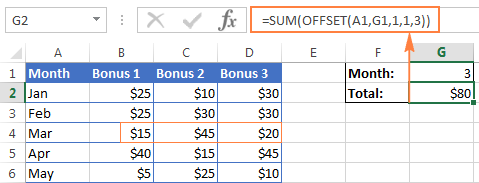
In situation when you wish to base the offset from the current cell, you can use the INDIRECT and ADDRESS functions in combination with ROW() and COLUMN() to get the starting reference. For example:
=SUM(OFFSET(INDIRECT(ADDRESS(ROW(), COLUMN())), 3, 1, 1, 3))
Why do I use OFFSET in Excel?
Now that you know what the OFFSET function does, you may be asking yourself "Why bother using it?" Why not simply write a direct reference like B4:D4?
The Excel OFFSET formula is very good for:
Creating dynamic ranges: References like B1:C4 are static, meaning they always refer to a given range. But some tasks are easier to perform with dynamic ranges. This is particularly the case when you work with changing data, e.g. you have a worksheet where a new row or column is added every week.
Getting the range from the starting cell. Sometimes, you may not know the actual address of the range, though you do know it starts from a certain cell. In such scenarios, using OFFSET in Excel is the right way to go.
How to use OFFSET function in Excel - formula examples
I hope you haven't get bored with that much of theory. Anyway, now we are getting to the most exciting part - practical uses of the OFFSET function.
Excel OFFSET and SUM functions
The example we discussed a moment ago demonstrates the simplest usage of OFFSET & SUM. Now, let's look at these functions at another angle and see what else they can do.
Example 1. A dynamic SUM / OFFSET formula
When working with continuously updated worksheets, you may want to have a SUM formula that automatically picks all newly added rows.
Suppose, you have the source data similar to what you see in the screenshot below. Every month a new row is added just above the SUM formula, and naturally, you want to have it included in the total. On the whole, there are two choices - either update the range in the SUM formula each time manually or have the OFFSET formula do this for you.
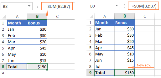
Since the first cell of the range to sum will be specified directly in the SUM formula, you only have to decide on the parameters for the Excel OFFSET function, which will get that last cell of the range:
Reference- the cell containing the total, B9 in our case.Rows- the cell right above the total, which requires the negative number -1.Cols- it's 0 because you don't want to change the column.
So, here goes the SUM / OFFSET formula pattern:
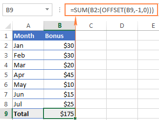
Tweaked for the above example, the formula looks as follows:
=SUM(B2:(OFFSET(B9, -1, 0)))
And as demonstrated in the below screenshot, it works flawlessly:
Example 2. Excel OFFSET formula to sum the last N rows
In the above example, suppose you want to know the amount of bonuses for the last N months rather than grand total. You also want the formula to automatically include any new rows you add to the sheet.
For this task, we are going to use Excel OFFSET in combination with the SUM and COUNT / COUNTA functions:
=SUM(OFFSET(B1,COUNT(B:B)-E1+1,0,E1,1))
or
=SUM(OFFSET(B1,COUNTA(B:B)-E1,0,E1,1))
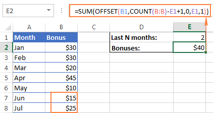
The following details can help you understand the formulas better:
Reference- the header of the column whose values you want to sum, cell B1 in this example.Rows- to calculate the number of rows to offset, you use either the COUNT or COUNTA function.COUNT returns the number of cells in column B that contain numbers, from which you subtract the last N months (the number is cell E1), and add 1.
If COUNTA is your function of choice, you don't need to add 1, since this function counts all non-empty cells, and a header row with a text value adds an extra cell that our formula needs. Please note that this formula will work correctly only on a similar table structure - one header row followed by rows with numbers. For different table layouts, you may need to make some adjustments in the OFFSET/COUNTA formula.
Cols- the number of columns to offset is zero (0).Height- the number of rows to sum is specified in E1.Width- 1 column.
Using OFFSET function with AVERAGE, MAX, MIN
In the same manner as we calculated the bonuses for the last N months, you can get an average of the last N days, weeks or years as well as find their maximum or minimum values. The only difference between the formulas is the first function's name:
=AVERAGE(OFFSET(B1,COUNT(B:B)-E1+1,0,E1,1))
=MAX(OFFSET(B1,COUNT(B:B)-E1+1,0,E1,1))
=MIN(OFFSET(B1,COUNT(B:B)-E1+1,0,E1,1))
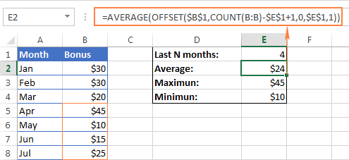
The key benefit of these formulas over the usual AVERAGE(B5:B8) or MAX(B5:B8) is that you won't have to update the formula every time your source table gets updated. No matter how many new rows are added or deleted in your worksheet, the OFFSET formulas will always refer to the specified number of last (lower-most) cells in the column.
Excel OFFSET formula to create a dynamic range
Used in conjunction with COUNTA, the OFFSET function can help you make a dynamic range that may prove useful in many scenarios, for example to create automatically updatable drop-down lists.
The OFFSET formula for a dynamic range is as follows:
=OFFSET(Sheet_Name!$A$1, 0, 0, COUNTA(Sheet_Name!$A:$A), 1)
At the heart of this formula, you use the COUNTA function to get the number of non-blank cells in the target column. That number goes to the height argument of OFFSET instructing it how many rows to return.
Apart from that, it's a regular Offset formula, where:
- Reference is the starting point from which you base the offset, for example Sheet1!$A$1.
- Rows and
Colsare both 0 because there are no columns or rows to offset. - Width is 1 column.
Note. If you are making a dynamic range in the current sheet, there is no need to include the sheet name in the references, Excel will do it for you automatically when creating the named range. Otherwise, be sure to include the sheet's name followed by the exclamation point like in this formula example.
Once you've created a dynamic named range with the above OFFSET formula, you can use Data Validation to make a dynamic dropdown menu that will update automatically as soon as you add or remove items from the source list.
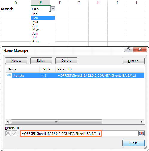
For the detailed step-by-step guidance on creating drop-down lists in Excel, please check out the following tutorials:
Excel OFFSET & VLOOKUP
As everyone knows, simple vertical and horizontal lookups are performed with the VLOOKUP or HLOOKUP function, respectively. However, these functions have too many limitations and often stumble in more powerful and complex lookup formulas. So, in order to perform more sophisticated lookups in your Excel tables, you have to look for alternatives such as INDEX, MATCH and OFFSET.
Example 1. OFFSET formula for a left Vlookup in Excel
One of the most infamous limitations of the VLOOKUP function is inability to look at its left, meaning that VLOOKUP can only return a value to the right of the lookup column.
In our sample lookup table, there are two columns - month names (column A) and bonuses (column B). If you want to get a bonus for a certain month, this simple VLOOKUP formula will work without a hitch:
=VLOOKUP(B1, A5:B11, 2, FALSE)
However, as soon as you swap the columns in the lookup table, this will immediately result in the #N/A error:
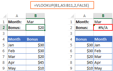
To handle a left-side lookup, you need a more versatile function that does not really care where the return column resides. One of possible solutions is using a combination of INDEX and MATCH functions. Another approach is using OFFSET, MATCH and ROWS:
Where:
- Lookup_col_offset - is the number of columns to move from the starting point to the lookup column.
- Return_col_offset - is the number of columns to move from the starting point to the return column.
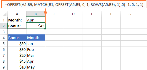
In our example, the lookup table is A5:B9 and the lookup value is in cell B1, the lookup column offset is 1 (because we are searching for the lookup value in the second column (B), we need to move 1 column to the right from the beginning of the table), the return column offset is 0 because we are returning values from the first column (A):
=OFFSET(A5:B9, MATCH(B1, OFFSET(A5:B9, 0, 1, ROWS(A5:B9), 1) ,0) -1, 0, 1, 1)
I know the formula looks a bit clumsy, but it does work :)
Example 2. How to do an upper lookup in Excel
As is the case with VLOOKUP being unable to look at the left, its horizontal counterpart - HLOOKUP function - cannot look upwards to return a value.
If you need to scan an upper row for matches, the OFFSET MATCH formula can help again, but this time you will have to enhance it with the COLUMNS function, like this:
Where:
- Lookup_row_offset - the number of rows to move from the starting point to the lookup row.
- Return_row_offset - the number of rows to move from the starting point to the return row.
Assuming that the lookup table is B4:F5 and the lookup value is in cell B1, the formula goes as follows:
=OFFSET(B4:F5, 0, MATCH(B1, OFFSET(B4:F5, 1, 0, 1, COLUMNS(B4:F5)), 0) -1, 1, 1)
In our case, the lookup row offset is 1 because our lookup range is 1 row down from the starting point, the return row offset is 0 because we are returning matches from the first row in the table.

Example 3. Two-way lookup (by column and row values)
Two-way lookup returns a value based on matches in both the rows and columns. And you can use the following double lookup array formula to find a value at the intersection of a certain row and column:
Given that:
- The lookup table is A5:G9
- The value to match on the rows is in B2
- The value to match on the columns is in B1
You get the following two-dimensional lookup formula:
=OFFSET(A5:G9, MATCH(B2, OFFSET(A5:G9, 0, 0, ROWS(A5:G9), 1), 0)-1, MATCH(B1, OFFSET(A5:G9, 0, 0, 1, COLUMNS(A5:G9)), 0) -1)
It's not the easiest thing to remember, is it? In addition, this is an array formula, so don't forget to press Ctrl + Shift + Enter to enter it correctly.
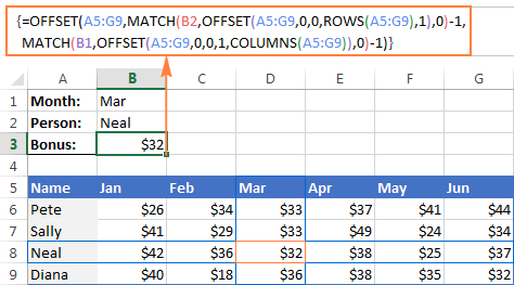
Of course, this lengthy OFFSET formula is not the only possible way to do a double lookup in Excel. You can get the same result by using the VLOOKUP & MATCH functions, SUMPRODUCT, or INDEX & MATCH. There is even a formula-free way - to employ named ranges and the intersection operator (space). The following tutorial explains all alternative solutions in full detail: How to do two-way lookup in Excel.
OFFSET function - limitations and alternatives
Hopefully, the formula examples on this page have shed some light on how to use OFFSET in Excel. However, to efficiently leverage the function in your own workbooks, you should not only be knowledgeable of its strengths, but also be wary of its weaknesses.
The most critical limitations of the Excel OFFSET function are as follows:
- Like other volatile functions, OFFSET is a resource-hungry function. Whenever there is any change in the source data, your OFFSET formulas are recalculated, keeping Excel busy for a little longer. This is not an issue for a single formula in a small spreadsheet. But if there are dozens or hundreds of formulas in a workbook, Microsoft Excel may take quite a while to recalculate.
- Excel OFFSET formulas are hard to review. Because references returned by the OFFSET function are dynamic, big formulas (especially with nested OFFSETs) can be quite tricky to debug.
Alternatives to using OFFSET in Excel
As is often the case in Excel, the same result can be achieved in a number of different ways. So, here are three elegant alternatives to OFFSET.
- Excel tables
Since Excel 2002, we have a truly wonderful feature - fully-fledged Excel tables, as opposed to usual ranges. To make a table from structured data, you simply click Insert > Table on the Home tab or press Ctrl + T.
By entering a formula in one cell in an Excel table, you can create a so-called "calculated column" that automatically copies the formula to all other cells in that column and adjusts the formula for each row in the table.
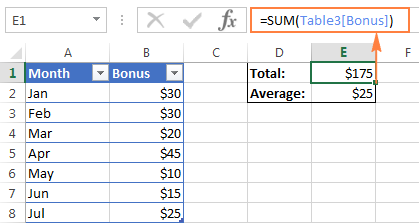
Moreover, any formula that refers to a table's data automatically adjusts to include any new rows you add to the table or exclude the rows you delete. Technically, such formulas operate on table columns or rows, which are dynamic ranges in nature. Each table in a workbook has a unique name (the default ones are Table1, Table2, etc.) and you are free to rename your table via the Design tab > Properties group > Table Name text box.
The following screenshot demonstrates the SUM formula that refers to the Bonus column of Table3. Please pay attention that the formula includes the table's column name rather than a range of cells.
- Excel INDEX function
Although not exactly in the same way as OFFSET, Excel INDEX can also be used to create dynamic range references. Unlike OFFSET, the INDEX function is not volatile, so it won't slow down your Excel.
- Excel INDIRECT function
Using the INDIRECT function you can create dynamic range references from many sources such as cell values, cell values and text, named ranges. It can also dynamically refer to another Excel sheet or workbook. You can find all these formula examples in our Excel INDIRECT function tutorial.
Do you remember the question asked at the beginning of this tutorial - What is OFFSET in Excel? I hope now you know the answer : ) If you want some more hands-on experience, feel free to download our practice workbook (please see below) containing all the formulas discussed on this page and reverse engineer them for deeper understanding. Thank you for reading!
Practice workbook for download
OFFSET formula examples (.xlsx file)
 by
by
93 comments
Hi, I am new to excel functions and would like to know how to handle a use-case with offset function as mentioned below:
I am trying to use the following generic formula with offset function in the very first row of my table. Since this is the first row, -A2 is giving the reference error. How can I handle it?
Here, A column holds the integer values and I wanted to use this formual to calculate the cumulative sum from the first day of a financial year (i.e., from April 1st and my table starts from January 1st)
D2=SUM(OFFSET(C2,0,0,-A2,1):C2)
Hi!
I don't really understand what you want to make your formula, what is written in cell A2, and what ":A2" means. Above in the article, there is an example of a sum with the OFFSET function.
Hi Alexander, I am computing YearToDate sales of a financial year(April 1st 2021 to March 31st 2022) in column D. And, Column C holds the sales value and Column A is a refernce column and it holds the number of the day in that financial year i.e., it holds 1 for April-1st-2021, 2 for April-2nd-2021 and so on. Since, my table is started from Jan 1st 2021, for that particular row, column A holds the value as 276 i.e., 276th day in the previous financial year.
I am using the offset function to make the starting point of YTD computation dynamic. Please let me know if you need any further clarification.
Col A Col B Col C Col D
276 01-Jan-21 5210 5200
277 02-Jan-21 5500 10710
Tried to show my table format below:
Col A |Col B |Col C |Col D
-------- -------------- --------- --------
276 |01-Jan-21 |5210 |5210
277 |02-Jan-21 |5500 |10710
Hello!
Please check out the following article on our blog, it’ll be sure to help you with your task: How to do a running total in Excel
I hope it’ll be helpful.
I have dates in one column that I want copied into another column and if one cell is empty ie no date then I want no entry in the 2nd column . The formula I set up works in the transfer of data with the exception that if there is no date in column "D" then it posts a date of 00-Jan-00 in column "H" and I want it just to be blank in column "H" I posted the following in column H
=offset($D$114,0,0,counta(D114:D250)*1) How can I correct this formula?
Hello!
If you want to replace zero with empty try this formula
=if(offset($D$114,0,0,counta(D114:D250)*1)=0,"",offset($D$114,0,0,counta(D114:D250)*1))
I hope it’ll be helpful.
1 TO 15 NUMBER IN COLUMN A
I WANT TO DISTRIBUTE LIKE THIS
1 6 11
2 7 12
3 8 13
4 9 14
5 10 15
Hello!
I’m sorry but your task is not entirely clear to me.
For me to be able to help you better, please describe your task in more detail. Please let me know in more detail what you were trying to find, what formula you used and what problem or error occurred. Give an example of the source data and the expected result. It’ll help me understand it better and find a solution for you. Thank you.
If Employee name is in column A, Emp ID in B. And in C, Status as (Active/Deactive). IN another sheet how to pull Emp id for active employees
Please share how to find last row in a column.
where
=LEFT(G9,5) returns $E$3
then =OFFSET(LEFT(G9,5),1,0) show error
where as =OFFSET($E$3,1,0) give an address
please say how to use
=OFFSET(LEFT(G9,5),1,0)
Is there a way to create an Excel table with a dynamic (formula-based) # of rows? For example, I'd like to build an amortization table, and I'd like to be able enter the # of months in a cell (e.g. 360 for a 30-year mortgage, 180 for 15-year mortgage, 60 for a 12-month car loan, etc) and then have a table with my amortization calculations populate based on the # of rows that I'm interested in.
Hello i have one query : i want to insert data and make one table according to this below equation for T COLUMN NUMBERS with the same interval. how can i do this kind of functionality in xlx
0 T3 T(3+8)=T11 T(11+8)=T19 T(19+8)=T27
10 T(3+128)=T131 T(11+128)=T139 T(19+128)=T147 T(27+128)=T155
20 T(131+128)=T259 T(139+128)=T267 T(147+128)=T275 T(155+128)=T283
30
40
50
60
70
80
90
A0
B0
C0
D0
E0
F0
100
Thank you so much for the information. It helped me a lot in several cases
=sheet1! B1
By dragging to down
=sheet1! B2
I want
=sheet2! B1
So please help me
=INDIRECT("'"&"Sheet"&ROW()&"'!B1").
When you copy and paste this formula down or drag it down, it should work.
Very Helpful Offset
Hi, how do I copy even cells in one column and odd cell in another column. Example value in cell B1 =A1, B2=A3 and C1=A2, C2=A4.
Thanks,
Hi,
I have around 10000 in one column , i would like do do shift every 100 rows then write the value and do on .
Thank you in advance
Hi,
I have around 10000 values in one column , i would like to do shift every 100 rows then write the value and do on .
Thank you in advance
Great info!!
I use OFFSET and Define Name to dynamically track the most recent 5 test results on a spreadsheet that expands over time.
=OFFSET('Test Results'!J6,1,COUNTA(‘Test Results'!$I$5:$DD$5)-5,1,-1)
The problem I run into is when entering the first few results. Any time there are less columns (or rows) with data than you have indicated in your OFFSET formula, the formula will reference irrelevant cells or produce errors if it runs out of columns (or rows).
For example, if my OFFSET is set to -5 (columns), but I only have 2 or 3 columns of data, my Offset formula will still try to reference 5 columns… so it will end up referencing column titles or whatever is to the left of my starting reference, or it will produce an error because there are no more columns remaining on the spreadsheet.
Is there a way to avoid this? Maybe some kind of parameter that tells it to stop at a specified column, or mixing in an IF, THEN formula?
Hello,
For me to understand the problem better, please send me a small sample workbook with your source data and the result you expect to get to support@ablebits.com. Please don't worry if you have confidential information there, we never disclose the data we get from our customers and delete it as soon as the problem is resolved.
Please also don't forget to include the link to this comment into your email.
I'll look into your task and try to help.
Lovely explanation
Thanks for that
Hi,
Need formula on below problem-
Column-"A"- Select-"YES"
Column-"B"- Select-"YES"
Column-"C" - SUM THE VALUE
It isn't true that the HEIGHT and WIDTH arguments of the OFFSET function must be positive (!)
I have played with your simple example of the SUM & OFFSET (where the result is displayed in cell G2), setting the above mentioned arguments to negative values.
Here are the results:
=SUM(OFFSET($A$1,3,3,-1,-1)) Result: 20
=SUM(OFFSET($A$1,3,2,-1,-1)) Result: 45
=SUM(OFFSET($A$1,3,2,-2,-2)) Result: 115
Excel accepted the negative values of the HEIGHT and WIDTH arguments, without any problem….
So, Microsoft's user's manual is probably wrong….
Anyone up for a super big challenge? Here is my formula: I need it OFFSET!
IF(SIN($D2)*SIN($G2)+COS($D2)*COS($G2)*COS($H2-$E2)> 1,3963.1*ACOS(1),3963.1*ACOS(SIN($D2)*SIN($G2)+COS($D2)*COS($G2)* COS($H2-$E2)))
HELP! Imagine a big data base that looks like this:
New York Chicago DC
New York to LA 1300 miles !!! !!! !!
Chicago to Boston 700 Miles
DC to Charlotte 300 Miles
OK So I want to create this big routing calculator in Excel. I have all of the GPS coordinates...I have the distance between routes, but I need to find out which one to do next...
So go to the New York to LA...You see it's 1300 Miles? Note going horizontally is New York, Chicago, and DC. I need to fill those in. So I need to copy that massive formula ACROSS, but I need the rows to go DOWN. Columns stay the same, rows go down using OFfset.
Any takers?
Anyone up for a super big challenge? Here is my formula: I need it OFFSET!
IF(SIN($D2)*SIN($G2)+COS($D2)*COS($G2)*COS($H2-$E2)> 1,3963.1*ACOS(1),3963.1*ACOS(SIN($D2)*SIN($G2)+COS($D2)*COS($G2)* COS($H2-$E2)))
Imagine a big data base that looks like this:
New York Chicago DC
New York to LA 1300 miles !!! !!! !!
Chicago to Boston 700 Miles
DC to Charlotte 300 Miles
OK So I want to create this big routing calculator in Excel. I have all of the GPS coordinates...I have the distance between routes, but I need to find out which one to do next...
So go to the New York to LA...You see it's 1300 Miles? Note going horizontally is New York, Chicago, and DC. I need to fill those in. So I need to copy that massive formula ACROSS, but I need the rows to go DOWN. Columns stay the same, rows go down using OFfset.
Any takers?
Excellent article. I make good use of the OFFSET() function including within the SUM() function, i.e. SUM(OFFSET()). I have today come across something that is baffling me. I am trying to use the OFFSET() function to define the range inside a SUMIF() function. When I use the construct on some small test data it works perfectly but when I put it to use on the full data set it only sums the first column. Here is the formula:
=SUMIF(A25:A160,A200,OFFSET(A25,0,958,ROWS(A25:A160),28))
Can anybody see the glaringly obvious that I am missing? It works fine if I use a similar construct as a SUM(). Or is there an unpublished limitation in the function?
(Using the ROWS() function ensures that everything will stay lined up if somebody inserts a row. 958 and 28 will be variables calculated in
other cells.)
Thank you.
Very helpful.
Just to say thanks for your Excel tips they are the best currently on the internet. I am currently using OFFSET and it is working very well.
Hi,
I need a excel formula that will arrange values in a row from differents columns but avoid 0(zero)value if in any cell.
Data in this format
A B C
1 24 15
13 0 6
To be arrange
A B C
1
24
15
13
6
Kindly awaiting your post
Hi,
I need a excel formula that will arrange values in a row from differents columns but avoid 0(zero)value if in any cell.
Data in this format
1 24 15
13 0 6
To be arrange
1
24
15
13
6
Kindly awaiting your post
Hello,
I have a spreadsheet with headings in column A. I would like to use a formula to to create a contiguous information - that is no unnecessary blank rows but I do need to keep all the headings in the rows.
Thank you.
Hi! This is an awesome forum and thank you for teaching me the offset function. It is working almost perfectly for me but I need to understand how to return the last 5 values in a single column of data and ignore the zeros... so my data looks like this - my offset calc is bringing back the last 5 values - but is bringing back 18, 16, 0, 17, 24 and I need to bring back 18, 16, 17, 24, 22... recommendations? Thank you so much!
Score
15
12
0
0
22
14
6
5
0
0
0
0
0
15
18
22
24
17
0
16
18
I am trying to create a sheet where the data is referenced from another sheet "Data_Sheet_name" and then creating multiple such coupled sheets using VBA. But every time I create a copy of the data sheet the referencing go haywire. So I want a formula which can dynamically be linked to the sheet based on the active sheet name.
Hi,
I have a spreadsheet with months 1,2,3 etc across the rows and a specific number of months to count backwards in a cell. For instance, I want to use the offset function to count back 6 columns from the reference cell. However, the 6 month count results in being either off the spreadsheet or into my column with all my field labels. This is causing the error either #value or #ref.. Unless I put the offset formula starting after column F (6 columns forward). How can I incorporate the offset function while not going off the sheet or into a cell that has text?
Thanks
Greg
Hey Greg, I'm having the same problem. Did you ever figure it out?
Hello, I have a problem which is not related to this tutorial. I am very new to excel, and I have learnt a lot from you. Thanks a lot. Suppose you have data in columns A1 to D20 and you want one formula to find minimum in every ROW and SUM the minimums. I have come across the following formulas in the internet, which I would kindly ask you to unravel me. I thank you in advance:
=SUM(MOD(LARGE(MAX(A1:D20+1)*ROW(A1:D20)+A1:D20,ROW(A1:D20)*COLUMNS(A1:D20)),MAX(A1:D20+1)))
=SUM(MOD(LARGE(100*ROW(A1:D20)+A1:D20,ROW(A1:D20)*COLUMNS(A1:D20)),100))
Excellent tutorials on Use of OFFSET Function.
Could you explain please how to use SUMIFS and Offset together in one formula. Thank you in advance.
hello there, I am trying to find the average of completion of TASKS CATEGORY based on the completion of individual TASKS.
I have 22 tasks in each table and a total of 3 main tasks category, and I am not able to return to average based on the product name.
The tab I am using has the same table repeating multiple times, one for each product I am working on. Each table has the same list of tasks to be performed with the following layout:
B1 is the name of the product (unique)
B4 to B25 is the list of tasks named p1....p22
c4 to c25 is the percentage value of progress for each task.
The table repeats itself underneath several times, what changes is the product name on b1, b27, b53, b79.. The tasks name (p1 to p22) are identical for each table in column b. I think the problem I am having is to return the average of the categories: tasks named p1 to p7 (cells b4 to b10) belong to the first category, tasks named p8 to p15 (cells b11 to b18) belong to the same category, and tasks named p16 to p22 (cells b19 to b25) belong to the third category. How do I get the average of the categories based on individual tasks completion % in column c based on the unique product name which is in b1, b27, b53, b79.. Thank you so much!!
Hi This one is a bit of a challenging one
I am not 100% sure if this uses the offset ruling or just the countif but i would really (really really really !!!) appreciate the advice.
My data set involves dates and times and I want to make a count of new events occurring in a separate column. A new event is classed as anytime the previous column has increased by 5 minutes.
Backgroud Info:
so the data is times and dates of pictures taken of animals and i have to make a count of every time an event happens.
An event is classified as any new animal that comes into view or if the same animal goes off camera and returns with over a 5 minute increase from the last time it was shown on camera.
So if it goes off camera and comes back under 5 minutes time(for example 4mins 31) i dont want to count it.
Further more, if another animal comes into view so 2 are in the shot i want to classify that as a new event also.
So for example :
date of shot time No.of animals in shot Event Counter
01.02.2016 10.50 1 1
01.02.2016 10.51 1
01.02.2016 10.51 1
01.02.2016 10.51 2 2
01.02.2016 10.51 1
01.02.2016 10.56 1 3
02.02.2016 16.51 2 4,5
02.02.2016 16.52 2
02.02.2016 16.58 1 6
02.02.2016 16.59 1
02.02.2016 17.05 1 ...formula???
so as you can see it is the end column i need the formula for to take into account date and time increase by 5 minute increases and an added count for if there is an extra animal in shot.
I have 15,000+ data points so if you can help me it would just be amazing.
The times only show shots of animals so theres no need to worry about an animal column.
fingers crossed you can help!Thanks
Respected Madam/Sir,
I found Tutorials on Using OFFSET function in Excel-formula examples, very useful and helped me to understand the offset function better.
Excellent detailed examples on offset.
Thanks a lot.
Regards,
P. G. Kerkar
hi,
i am facing an issue in excel how can i merge these two colums in one cell in top to down maner.
fr eg:- ram shayam amit
i want this in one cell like ram
shayam
please help its urgent!!!
Hi All,
Excellent examples and discussions on OFFSET.
How can you ensure that the cell format is the same when using OFFSET. For e.g., the OFFSET works, it returns the value of the cell to the appropriate new location, but some of my original cells are text hyperlinks (URLs). Thus, OFFSET only returns the text and it is not hyperlinked. Is this achievable?
Thank you.
Hi All,
Hopefully I am in the right spot for this question..
Basically I want to count the number of times a certain number appears in the last 20 results in a list - the list is updated often, so last 20 results changes.
RESULT NUMBER # APPEARANCES
3 1 ?
10
7
7
4
10
2
2
1
11
5
11
4
2
8
4
7
Appreciate any assistance you can give.
Hi,
Great summary on Offset, just one question that can I use offset in two different excel workbook?
Hi Xian,
Yes, it can. For example, this formula will return a value from cell B4 in Sheet1 of Book2:
=OFFSET([Book2]Sheet1!A1,3,1)
Hi,
A BIG thanks for this clarification. However, I need your help in the following issue: OFFSET function returns the value of a specific cell. How can I get the value next to that cell, and the one next to it, and the one next to it, etc. In other words, I need your help in the following: As I go to the right, I want to get the values of certain cells that go downwards.
Hope that is clear. I really appreciate your help.
I have a variable value in C6 which should be matched with the value in E6. C6 depends on the value in A2 not directly but indirectly.
I want the excel to auto calculate A2, for any given value in E6, such that C6=E6.
good article!
Thank you for your help. I can now view well the function of Offset as compared to Index and Vlookup.
I'm a self trainee with good progress
Hi,
My challenge is to retain the same format ( including color of the cell value) when I do a offset. Could anyone help me with this. Thanks
I ran into an interesting problem with the offset function:
I have a table with string data containing newlines. For example:
this
is
my
data
the above would all be in 1 cell, but with 1 word per line and a new line character after each word (by pressing alt+enter). This works great, but if I use the offset function and it selects that cell, I get "thisismydata" with no newline characters in it.
Any tips?
This post is very insightful indeed. I have learned a lot. Many thanks!
Also, kindly help me with a simple formula on this:
I have an excel data that I use to monitor attendance at meetings. The columns labelled YES/NO tell whether the meeting was held or not. I want to monitor attendance in the last N meetings held (eg.last 2 or 3 columns with a "YES"). It should not count the cell when the column heading is "NO".
That is: if I enter 2 in cell H2 it should return (2 in H3 for Mr. A and 1 in H4 for Mr. B etc). if I enter 3 in H2 it should return (3 in H3 for Mr. A and 2 in H4 for Mr. B etc)
A B C D E F G H
1 Jan15 Feb-15 Mar-15 May-15 Jun-15 Jul-15 Last N meetings
2 Name YES YES NO YES NO YES
3 Mr.A 1 1 1 1
4 Mr.B 1 1 0 1
5 Mr.C 0 1 1 1
6 Mr.D 0 1 1 1
7 Mr.E 1 1 0 1
Thank you
Hello, Prince,
Sorry, it's difficult to create a formula according to your example. Could you sand us a small sample table in Excel to support@ablebits.com?
Thanks for this email. I need your help.
I want a formula to search for certain strings located in a column in one sheet from a column in another sheet and replace the content of the column in the second sheet with that of the string from the first sheet if found.
i.e. if 'xyz' in cell A1 of sheet test if found in 'sjkhgjjhkxyzrewqed' of cell b3 in sheet test2 replace 'sjkhgjjhkxyzrewqed' with 'xyz'.
Thanks to your expected help.
Regards
hi, i understand that you want to replace sheet2 b3 cell should be enter as sheet1 a1 value
in that case you can use these formulas in sheet2 b3 cell
those are
1) =xyz!A1
2)=indirect("xyz!A1")
here "xyz" means sheet1 name
Hope you find the solution
or else please let me know
Hi
I have to 2 excel sheet.
Sheet A :The value for average of differnt columns in different cells but in same row G41.(average of column c in c41;average of column G in G41;average of column J in J41 and so on )set repeats after every 6 columns.
Now in sheet "B" I want all the results of sheet A in column H one after other .(I cant drag the formula as the range is not continues). Please help
Hi!, I want to thank Oyu in advance.
I use this function to count the number of zeros after the last non zero data. It works perfect, except when the first cell in the row is zero.
COLUMNS(D24:W24)-MATCH(2;1/(D24:W240))-COUNTBLANK (D24:W24)
I want the formula to start counting zeros from the first cell if it is zero.
Thanks
Hello, Ahmed,
For us to be able to assist you better, please send us a sample table with your data in Excel to support@ablebits.com.
=SUM(OFFSET(H4,0,0,1,-$L$3))
Hey, I just wanted to say that I really appreciate you putting this together. I'm sure it involved quite a bit of work!
Thanks so muchh!