This tutorial will guide you on how to make a checkbox in Excel and use the check box results in formulas to create an interactive checklist, to-do list, report or graph.
I believe everybody knows what a checkbox is, you must have seen plenty of them on various forms online. Still, for the sake of clarity, let me begin with a brief definition.
A check box, also referred to as a tick box or checkmark box or selection box, is a little square box where you click to select or deselect a given option.
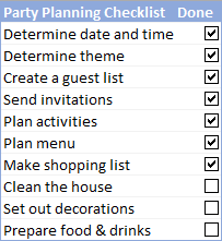
Inserting a checkbox in Excel sounds like a trivial thing, but it opens up a host of new possibilities for your worksheets that will keep you on track with your goals, schedule, assignments, etc.
How to insert checkbox in Excel
Like all other Form controls, the Check Box control resides on the Developer tab, which does not appear on the Excel ribbon by default. So, you need to turn it on first.
1. Show the Developer tab on the ribbon
To add the Developer tab to the Excel ribbon, do the following:
- Right-click anywhere on the ribbon, and then click Customize the Ribbon… Or, click File > Options > Customize Ribbon.
- Under Customize the Ribbon, select Main Tabs (usually it is selected by default), check the Developer box, and click OK.
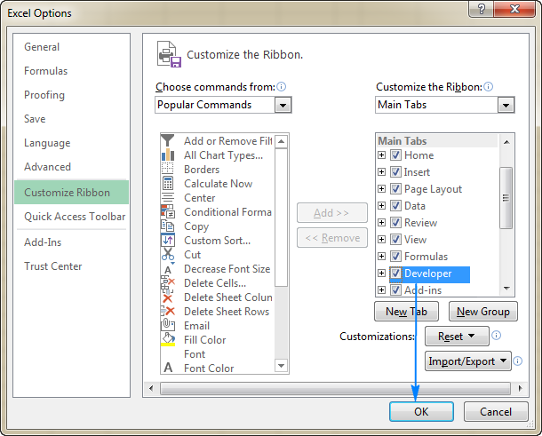
Now, with the Developer tab in place, you get access to a host of interactive controls, including Check Box.
2. Organize the data
If you are creating an Excel checklist or to-do list, the first step is to make a list of tasks or other items for which the check boxes will be inserted.
For this example, I've created the following Party Planning Checklist:
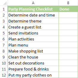
3. Add a check box
The preparation steps are completed, and now we are getting to the main part - add checkboxes to our Party Planning list.
To insert a checkbox in Excel, execute these steps:
- On the Developer tab, in the Controls group, click Insert, and select Check Box under Form Controls.
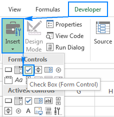
- Click in the cell where you want to insert the first checkbox (B2 in this example). The Check Box control will appear near that place, though not exactly positioned in the cell:
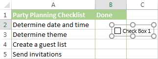
- To properly position the check box, hover your mouse over it and as soon as the cursor changes to a four-pointed arrow, drag the checkbox where you want it.

- To remove the text "Check Box 1", right click the checkbox, select the text and delete it. Or, right click the check box, select Edit Text in the context menu, and then delete the text.
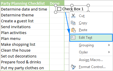
Your first Excel checkbox is ready, and you just have to copy it to other cells.
4. Copy the checkbox to other cells
Select the cell with the check box by using the arrow keys on your keyboard, and position the cursor over the lower right corner of the cell. When the mouse pointer changes to a thin black cross, drag it down to the last cell where you want to copy the checkbox.
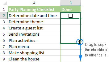
Done! The check boxes are added to all the items in the checklist:
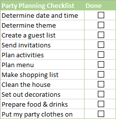
As you can see in the screenshot above, our Excel checklist is almost ready. Why almost? Although the checkboxes are inserted and you can now check or uncheck them by simply clicking on a box, Microsoft Excel is not able to respond to these changes because no cell is linked to any of the checkboxes yet.
The next part of our Excel Checkbox tutorial will teach you how to capture the user selecting or clearing a checkbox and how to use that information in your formulas.
How to link a checkbox to a cell
As already mentioned, to be able to capture the checkbox state (checked or unchecked) you need to associate the check box with a certain cell. To do this, please follow these steps:
- Right click the checkbox, and then click Format Control.
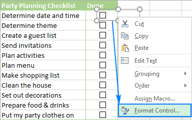
- In the Format Control dialog box, switch to the Control tab, click in the Cell link box and select an empty cell on the sheet to which you want to link to the checkbox, or type the cell reference manually:
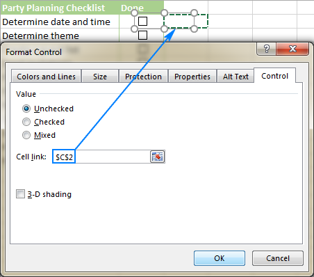
- Repeat the above step for other check boxes.
Tip. To easily identify the linked cells, select them in an adjacent column that does not contain any other data. This way, you will be able to safely hide the linked cells later so they won't clutter your worksheet.
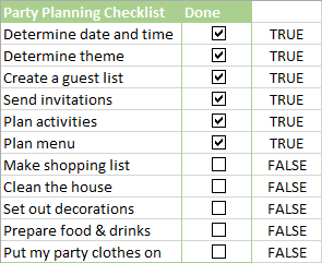
- Finally, click on each of the linked checkboxes. In the linked cells, TRUE appears for selected checkboxes, and FALSE for cleared checkboxes:
At this point, the linked cells probably don't make much sense, but please bear with me just a little longer and you will see how many new opportunities they provide to you.
Examples of using checkboxes in Excel
Below you will find a few examples of how to use checkboxes in Excel to make an interactive checklist, to-do list, report and chart. But first, let's learn how to link checkboxes to cells. The technique is very simple, but it's the corner stone of using the checkbox results in your formulas.
Tip. To quickly get a selection of checklist templates for Excel, click File > New, type "checklist" in the search box, and press Enter.
How to make a checklist with data summary
In fact, we have already done the major part of the job by adding check boxes and linking them to cells. Now, we will just write a few formulas to create a data summary for our Excel checklist.
Formula to calculate the total number of tasks
It's the easiest one - use the COUNTA function to get the number of non-blank cells in the checklist:
=COUNTA(A2:A12)
Where A2:A12 are the checklist items.
Formula to count the number of checkmarked items (completed tasks)
A completed task means a checkbox with a tick symbol in it, which means the TRUE value in a linked cell. So, get the total count of TRUE's with this COUNTIF formula:
=COUNTIF(C2:C12,TRUE)
Where C2:C12 are the linked cells.
To make a formula a bit more clever, you use COUNTIFS instead of COUNTIF to check for blank cells in the list (column A):
=COUNTIFS(A2:A12, "<>", C2:C12, TRUE)
In this case, if you delete some irrelevant item(s) from your Excel checklist, but forget to remove a check symbol from the corresponding box, such checkmarks won't be counted.
Formula to get the percentage of completed tasks
To calculate the presented of the tasks completed, use the regular percentage formula:
Part/Total = Percentage
In our case, divide the number of completed tasks by the total number of tasks, like this:
=COUNTIF(C2:C12,TRUE)/COUNTA(A2:A12)
The following screenshot demonstrates all of the above formulas in action:
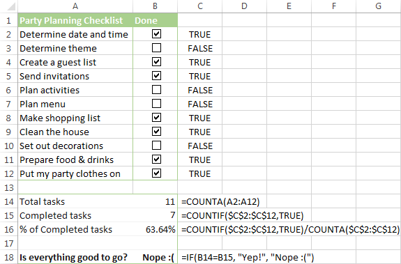
As you can see in the screenshot above, we have inserted one more formula in B18. The formula is based on the IF function that returns "Yes" if the number of completed tasks is equal to the tasks total, "No" otherwise:
=IF(B14=B15, "Yep!", "Nope :(")
To embellish your checklist a bit further, you can create a couple of conditional formatting rules that will change the color of cell B18 depending on its value.
Once that's completed, hide the column with linked cells, and your Excel checklist is done!
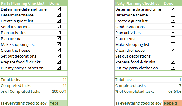
If you like the checklist we've created for this example, you are welcome to download it now.
How to create a To-Do list with conditional formatting
Basically, you can add checkboxes and formulas for a to-do list exactly in the same way as we have just done for the Excel checklist. "What's the point of writing this section then?" you can ask me. Well, in a typical to-do list, the completed tasks have the strikethrough format like this:
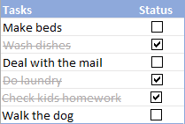
This effect can be easily achieved by creating a conditional formatting rule. The detailed steps follow below.
To begin with, write down a list of tasks, insert checkboxes and link them to cells:
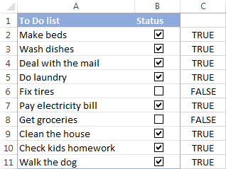
And now, apply conditional formatting that will give the strikethrough format and, optionally, a different background or font color to the checked items.
- Select a list of tasks (A2:A11 in this example).
- Go to the Home tab > Styles group, and click Conditional Formatting > New Rule…
- In the New Formatting Rule dialog box, select Use a formula to determine which cells to format.
- In the Format values where this formula is true box, enter the following formula:
=$C2=TRUEWhere C2 is the top-most linked cell.
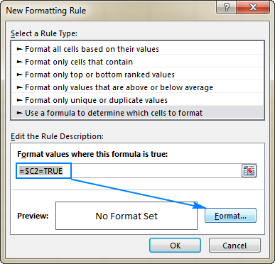
- Click on the Format button, set up the desired formatting style, and click OK. In this example, we select the Strikethrough effect and the light grey font color:
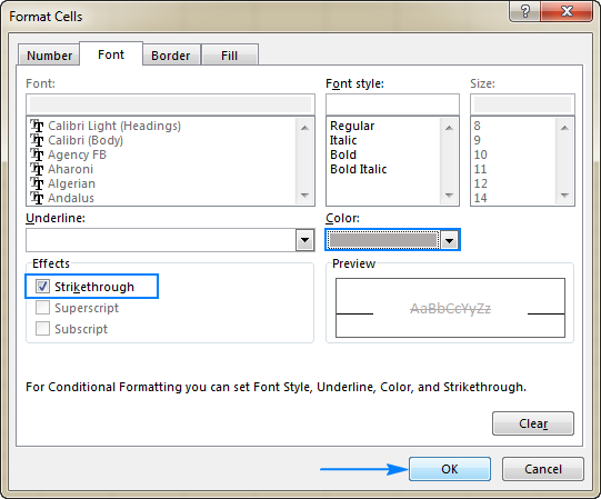
Tip. If you have little experience with conditional formatting, you may find the following detailed guidance helpful: Excel conditional formatting based on another cell value.
As of now, whenever a certain box is checked, the corresponding item gets formatted in the light grey font color with a strikethrough.
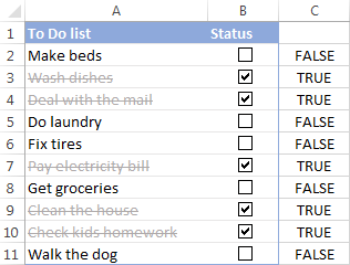
And here's one more idea for formatting your Excel to-do list. Instead of crossing out the competed tasks, you can insert an additional column with the following IF formula:
=IF(E2=TRUE, "Done", "To Be Done")
Where E2 is the top-most linked cell.
As shown in the screenshot below, the formula returns "Done" if a linked cell contains TRUE, "To be done" if FALSE:
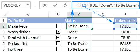
After that, apply the desired conditional format to the Status column based on this formula:
=$C2="Done"
The result will look something similar to this:
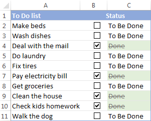
Lastly, add a couple of formulas to calculate the completed tasks (like we did for the checklist), hide the linked cells, and your Excel To Do list is good to go!
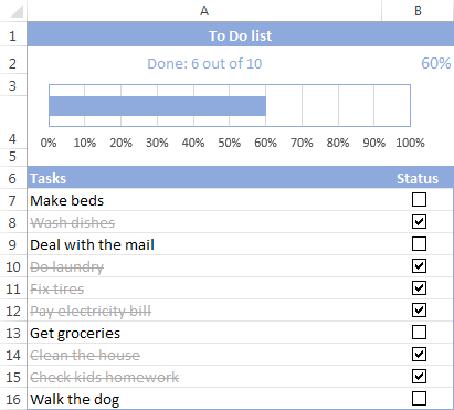
The bar chart at the top of the To-Do list is based on the percentage formula in B2. If you are curious to know the details of creating such a checklist with completion percentage bar, I encourage you to download the template, unhide columns D and E, and investigate the formulas.
How to create an interactive report with check boxes
Another useful application of checkboxes in Excel is for creating interactive reports.
Supposing you have a sales report that includes data for 4 regions: North, South, East and West. Your aim is to get the total for one or more selected regions. Of course, this can be done by using the Slicers feature of an Excel table or PivotTable or by inserting Subtotals. But why don't we make the report more user-friendly by inserting 4 checkboxes at the top?
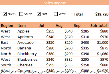
Looks nice, isn't it? To create a similar report in your sheet, please follow these steps:
- Add 4 checkboxes at the top of the sheet, for the North, South, East and West regions.
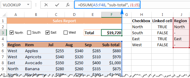
- Create the criteria area somewhere in an unused part of the sheet, and link the checkboxes to empty cells:

In the above screenshot, I2:I5 are linked cells and H2:H5 are the region names exactly as they appear in the report.
- Add one more column to the criteria area with an IF formula that returns the region name if the linked cell evaluates to TRUE, a dash ("-") otherwise:
=IF(I2=TRUE, H2, "-")
- Type a heading for the formula column that exactly matches the heading of the corresponding column in the report (Region in this example). The exact match is very important and on the next step, you will understand why.
- Next, write the formula to calculate the total for selected regions. For this, we are going to use the DSUM function that sums the values in a database that match the specified conditions:
DSUM(database, field, criteria)
Where:
- Database is your table or range including the column headings (A5:F48 in this example).
- Field is the column you want to sum. It can be supplied either as the column heading enclosed in the quotation marks, or a number that represents the position of the column in the database. In this example, we add up numbers in the Sub-total column, so our second argument is "sub-total".
- Criteria is the range of cells that contain your conditions, including the column heading (J1:J5). That is why the heading of the formula column in the criteria area should match the column heading in the report.
Put the above argument together, and your DSUM formula goes as follows:
=DSUM(A5:F48, "sub-total", J1:J5)…and works perfectly!
If you'd like to hide the #DIV/0! error that appears when no region is selected, wrap DSUM into the IFERROR function:
=IFERROR(DSUM(A5:F48, "sub-total", J1:J5), 0)
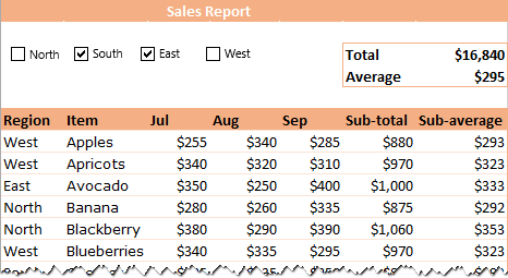
If in addition to total, your report calculates an average for each row, you can use the DAVERAGE(database, field, criteria) function to get a sales average for the selected regions.
Finally, hide and probably lock the criteria area to prevent accidental changes, and your interactive report is all set!
Make a dynamic chart based on the checkbox state
This example will teach you how to create a dynamic Excel chart that can respond to changing the checkboxes state (selected or cleared):
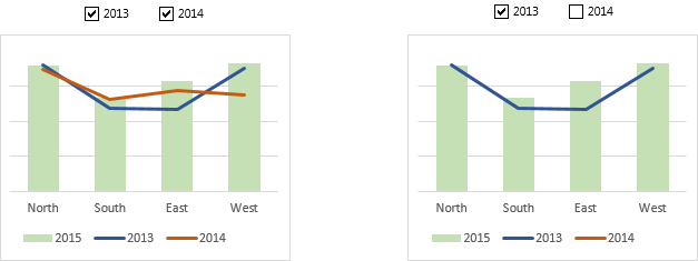
The source data for this example is as simple as this:
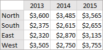
To turn it into a dynamic Excel graph, execute the following steps:
- Create checkboxes and link them to empty cells.
In particular, insert 2 checkboxes for the 2013 and 2014 years, and connect them to cells G2 and G3, respectively:
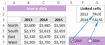
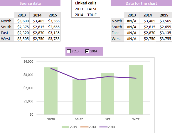
- Create the dataset for the chart dependent on the source data and linked cells (please see the image below):
- For 2013 year (J4:J7), use the following formula:
=IF($G$2=TRUE, B4, NA())If the 2013 checkbox is selected (G2 is TRUE), the formula pulls the original value from B4, otherwise returns the #N/A error.
- For 2014 year (K4:K7), enter a similar formula to pull the values from column C if the 2014 checkbox is selected:
=IF($G$2=TRUE, C4, NA()) - In cell L4, enter the formula
=$D4, and copy it down to L7. Because the data for the year 2015 should always be displayed in the chart, an IF formula is not needed for this column.

- For 2013 year (J4:J7), use the following formula:
- Create a combo chart based on the dependent data set (I3:L7). Since we have linked all cells in the dependent table to the original data, the chart will update automatically as soon as any change has been made in the original data set.
This is how you can create and use checkboxes in Excel. To review all the examples discussed in this tutorial, you may want to download our sample workbook below. I thank you for reading and hope to see you on our blog next week.
Practice workbook for download
Excel Checkbox examples (.xlsx file)
 by
by
100 comments
I have a list I created in Worksheet 2, that is used to create the dropdown list in Worksheet 1. What I am trying to do is when a selection is made from the dropdown list, I want the associated checkbox next to the selected item in the dropdown list to be checked. In this context, we are creating a buyout tracking list. I am in the construction industry and want to use this as a way to track my buyouts and know what is still open without having to do it by hand. Any suggestions? Everything I have tried has failed - miserably. :-(
Here is the list was created on Worksheet 2 with the check-boxes in adjacent cells. When the selection is made on Worksheet 1, I want the checkbox to populate on Worksheet 2.
if I wanted to use 2 check boxes one as yes and one as no for example is there a way of only 1 being checked at a time?
I cannot get the cells to carry the checkbox down to cells below once inserted.
I have tried hovering over the bottom RH corner and dragging on the cross as per the instructions (like normally in excel), and it doesn't work for me.
how do I fix this?
Hi Bradyn,
For a checkbox to get copied, it is important that the mouse pointer changes to a black cross when hovering over the bottom right corner of a cell (like shown in the screenshot in this post).
If it still doesn't work, please try one of the methods described in How to insert multiple checkboxes in Excel (copy check boxes).
Svetlana ur hot.how to clear check box once unticked
Hi Amir,
If you want to delete a checkbok, here's what you do:
- Select the checkbox (alick on the checkbox while holding the Ctrl key).
- Press the Delete key on your keyboard.
If you are asking about something else, please clarify.
Thank you very much!
Hi, I am trying to build a quote sheet to where if I check the check box it will show me the value of the option chosen versus true or false. Is that something that can me done?
Example:
Microwave $100 check box (if checked would = to the microwave total in a different cell
Thank you so much for your help
We have 100's of check boxes and any shortcut to apply cell link
This has been incredibly useful. Thank you :-)))
All that I want is a simple checkbox in a simple cell. A lot of hoo ha in the explanation, and Excel menus are SO cluttered, it takes an extraordinary weird person to find stuff.
How about a simple "Add, Checkbox" !!!
Ridiculous !!!!!!!!!!
And Certainly:
"Unfortunately, due to the volume of comments received we cannot guarantee that we will be able to give you a timely response. When posting a question, please be very clear and concise. We thank you for understanding!"
Gee effen wizzzz !!!
In the explanation of how to create an interactive report with check boxes,
the DAVERAGE formula should be wrapped by IFERROR in order to avoid division by zero [#DIV/0!] when no region is chosen.
It should read:
=IFERROR(DAVERAGE($A$5:$G$49,"Average",$J$1:$J$5),0)
instead of:
DAVERAGE($A$5:$G$49,"Average",$J$1:$J$5)
Hi Meni,
Good point, thank you! Added the remark to the tutorial.
Thank you :)
This is very helpful, but the checkboxes don't appear to work when using grouping and/or filters. The checkboxes don't remain with the line they are attributed to. Any ideas?
guys Im using vb so 'd like to use check box to select item from the sheet then label will caption the selected item in the userform...
You can link the check box to the same cell you are placing the check box and use a font color to hide the value.
You can use a formula to obtain a TRUE/FALSE result and the check box will be checked if formula = TRUE and unchecked if FALSE (so it autofills)
@Zubair Checkboxes are objects, you can place them wherever you want
How do I add multiple developer checkboxes in one cell
Excellent article! Exactly what I needed to know, clearly explained and illustrated! Thank you SO much!
~ Gwen
If I have checklist of 300 points, will i have to repeat step of 'Format Control'--> 'Cell Link 300 times' ??? If yes than aaahhhhh
Hello,
I hope you are well!
Thank you very much for this tutorial, very very helpful.
I do have a quick question for you.
For the step: How to link a checkbox to a cell, any way to apply that to all check boxes ? I'm asking because I have a few thousand rows & check boxes, you can imagine how long that would take me to format each check boxes to link them to the associated cell.
Spasibo Svetlana, greatly appreciated!
Is it possible to excel in a dropdown list by making multiple selections with check box?
Hi,
I have inserted a check box in column 'A' via the 'developer' tab and it works ok.
Only problem is that when column 'B' - (which has the 'wrapped text'setting applied) -has text entered and it wraps the text, the column 'A' with the check box suddenly makes a extra check box within the same cell.
Any ideas why this may be please?
Thank you
I found your tutorial very helpful! It's very easy to generate the checkbox and customize filtering based on results. In my spreadsheet, I am anticipating data entry into another cell after the checkbox formatting. It looks like when new data is entered and if that data increases the size of the row, the checkbox does not move with the cell. It would be awesome if cell formatting could be accepted by the checkbox. Have you found this to be an issue or do you have a solution?
Thank you for the tutorial, very informative.
OI also need a similar solution as "Diana C" To have a series of checkboxes, but only 1 box can be selected per each row, eg: either "Male" or "Female", or also a multiple range such as "Married", "Single" "Divorced" or "Widowed" but only 1 box can be checked
If I have to add another line item within my list, is there a way to reorder them (A-Z for example) and keep my checkboxes with the line item, not the line row? When I sort, I lose my true/false data to the original row.
Is there a formula to make the check box check automatically if a cell is filled out. For example check box in a4, I want it to check if I put info in cell a3 otherwise leave blank if that cell is blank.
Might be easier NOT to use a Checkbox. Just use COUNTBLANK which also counts zero-length strings (e.g. "") sometimes left as a result from a formula as blanks so this is a valid alternative depending on the data layout
Example:
In A4 type (or paste): A3 Has Data
In B4 type (or paste): =COUNTBLANK(A3:A3)=0
B3 Will now show 'FALSE'
In A3 type some data (or paste): 123ABC
B3 Will now show 'TRUE'
Use Cell 'Conditional Formatting' on B4, select Red = 'FALSE' and Green = 'TRUE'
or you could put the formatting instead on A4 BUT linked to B4 being either FALSE or TRUE as above... and then hide B column.
Have left =COUNTBLANK(A3:A3)=0 range as A3:A3 a 'range of 1' but could be changed to any range, but obviously this means that all cells in the range would have to have data present.
If you need the reverse, change =0 to =1 to get FALSE = Data Present.
No check boxes to tick, no having to remember, its automatic, its reminding you all the time! until you enter some data!
Hope this helps
Hi Svetlana. Thanks for this info. Just wanted you to know your tutorial is still getting mileage!
Thank you Mark!
I am attempting to place a check box on my spread sheet that when it is checked, it will ignore or delete the contents of another box in a formula. I am not having much luck. Any suggestions?
Very helpful article, I learned many new things, thank you!
I have an additional question though. I'm trying to build something like a form, where people would tick, let's say the "Male" or the "Female" box. Is there a way to add a restriction so that people would be unable to check both boxes? So when they click on one box, it gets checked, but if after that they click on the second box, the second gets checked while at the same time the first gets unchecked.
Thank you in advance!
Hi
I have a task to do.
I've got list of parts in excel - number, name and symbol.
I wish that i mark checkbox in the line with one of part number -> part number will be copied to another place with name and symbol - how it is possible to make ?? -> I'm an enginier and sometimes I have to order parts for my machines. It would be nice if someone will share knowledge with me - or give me solution.
Thanks.
Hello,
I'm afraid there's no easy way to solve your task with a formula. Using a VBA macro would be the best option here.
However, since we do not cover the programming area (VBA-related questions), I can advice you to try and look for the solution in VBA sections on mrexcel.com or excelforum.com.
Sorry I can't assist you better.
Hi,
The checkboxes are a great tool, but I have a problem. I have like 1000 checkboxes in my file, do I need to link them to a cell one by one? Its a to do list that the employees must fill in for every job. So its the same list always repeating itself. But when I copy/paste it, and I click on the checkbox of the first job, the checkbox of the second job is also selected..
Hi Anthony,
Unfortunately, it is not possible to link checkboxes to cells in bulk. You can only do this individually for each checkbox.
I have a template to utilize each month and I would like to clear the checkbox each month and utilize the list again.
is this possible?
Thank u so much
Awesome! Thank you so much. Great tutorial!
how to create drop down list to open different different data or sheet in excel 2016.
how to hyperlink in a cell by using if function to open the different data.
Hi,
Can you help me??
how to insert tick mark in Excel 2007.
Regards,
Netrapal Yadav
hi Svetlana
how i can control checkbox size and position
thanks
Hi Hussam,
The easiest way to resize a checkbox is drag the sizing handles using the mouse. Or, you can right-click the checkbox, and then click Format Control... > Size.
To fix the position of a checkbox in the sheet independently from the cells, right-click the checkbox, click Format Control > Properties, and select the "Don't move or size with cells" option.
I noticed your checkboxes are larger than what actually occurs when adding the Checkbox form control in my version of excel (checkbox is extremely small in my version. How are you able to resize the box itself? What version of Excel are you using, maybe that is the difference. Kindly, Mia
Hello, Mia,
if the problem with your checkboxes isn't gone and you still need our assistance, please, email us at support@ablebits.com with a screenshot of your checkboxes and the info about your Excel and Windows versions that you're currently using. Don't forget to link this article and your commentary number in your email letter. We will get back in touch.
Hi Mia,
I used Excel 2013, and these are the default checkboxes, I did not resize them.
To resize a check box, right-click it, click Format Control, switch to the Size tab, and set the desired size.
In the example above, is there a way to combine 2 criteria? For example, what is the total of avocados sold in East region? Or any other similar combination?
Thank you for this very useful information!
Svetlana;
This is close to what I'm trying to do. I want to create a list of instructions depending on the outcome of a check box. So clicking one check box in say C1 would display a long list of To Do's in another column.
The list is built from numerous rows on another sheet of ideally from a "library" of text boxes for different tasks.
I have a list of say 10 questions with Yes/No check boxes. If an answer is yes, I want to display a predefined list of "To Do's" from a given textbox or table.
Can you help me find the answer??
THANK YOU!
I'm trying to do this as well. Any insight will be greatly appreciated!
Hello!
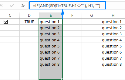
I think you can use the following approach:
- Link check boxes to some cells (say, link a checkbox in C1 to cell D1), the column of linked cell can be hidden later.
- Use the IF function to pull a list of To-Do's or other entries depending on the value in the linked cell (please mind the use of absolute and relative cell references in the formula):
=IF(AND($D$1=TRUE,H1<>""), H1, "")
Where D1 is a linked cell and H1 is the first entry of the list to be pulled.
The screenshot below shows a "prototype":
Thank you!!!! This is VERY helpful!
how to delete excell cell or row with check box in excel 2013
I need some help: I have multiple check boxes in multiple rows. I have 6 check boxes going across the spreadsheet. I'm having difficulty with: If all check boxes are checked then TRUE. If a check box is NOT checked, then FALSE. Any suggestions are greatly appreciative.
Ideally, I want to track which person has which items. If a person has all items, then it's good. If a person does not have all the items then I know I need to do some follow up.
Thanks,
Steve
very good tips. I am using the above tips. I will be grateful, if, I will guided how the "to be done lists" will be automatically forwarded to my email as a reminder.
Regards.
Rajanikanta
Hi Svetlana,
Yes, I found the way... I would like to put the number above the speedometer chart but I could not put the box above the chart (with the value link to the cell). Instead of that I used the chart title which links to the cell. Therefore once the value of the cell changes, the value inside the chart title also changes.
Thank's
Hi Svetlana,
I tried to make a box which shows the value from another cell. Therefore the value links to the cell.
Could you please to tell me how to link the value in the box to the cell?
Thank you
Hello Widojo,
In the Checkbox control, you can only put a tick mark and nothing else. Please consider creating a drop-down list instead based on the desired cells.
Hi,
Is there a way to make a check box cycle through a tick, a cross and blank through clicking the check box?
Thank you for this extremely interesting and useful tutorial. One observation I have is that it is quite laborious linking the Format Control dialog box to cell references - they have to be done individually - if you have a long list this could take a while! Is there an easy way round this?
Thanks
Bill
Hi William,
I guess there is no way other than VBA to link multiple Form Controls. For example, you can use this macro to link multiple check boxes:
http://www.pcreview.co.uk/threads/multiple-and-i-mean-multiple-checkboxes.1023995/
I just did the VBA method and it was very easy and useful!
IF D33= Rwanda,Kenya,(FREE),Tanzania,Uganda,Kenya,CPS,Tanzania, then AE = 1350
IF D33= Rwanda,Kenya,(FREE),Tanzania,Uganda,Kenya,CPS,Tanzania & IF F33 less than April 2016 then AE = 1300
IF D33= Rwanda,Kenya,(FREE),Tanzania,Uganda,Kenya,CPS,Tanzania & IF F33 greater than April 2016 then AE = 1350
IF D33= Rwanda,Kenya,(FREE),Tanzania,Uganda,Kenya,CPS,Tanzania & IF I33 less than April-24- 2016 then AE = 1300
IF D33= Rwanda,Kenya,(FREE),Tanzania,Uganda,Kenya,CPS,Tanzania & IF I33 greater than Oct- 2014 then AE = 1300
IF D33= Rwanda & I33=June-2015 then AE=700
Can you help me to set below formula.
Formula criteria
Set Formula in cell AE33
IF D33= Rwanda,Kenya,(FREE),Tanzania,Uganda,Kenya,CPS,Tanzania, then AE = 1350
IF D33= Rwanda,Kenya,(FREE),Tanzania,Uganda,Kenya,CPS,Tanzania & IF F33 April 2016 then AE = 1350
IF D33= Rwanda,Kenya,(FREE),Tanzania,Uganda,Kenya,CPS,Tanzania & IF I33 Oct- 2014 then AE = 1300
IF D33= Rwanda & I33=June-2015 then AE=700
The checkboxes for the interactive report & the dynamic charts are the equivalent of slicers, provided your data are in an Excel Table. Isn't it easier to use slicers?
Dear Klaas,
Thank you for your comment. Sure, slicers are very easy to use if your data is organized in a table or PivotTable. But this tutorial targets check boxes and I wanted to demonstrate a few uses other than conventional check lists and to-do lists.