The tutorial explains how to use the Excel Subtotal feature to automatically sum, count or average different groups of cells. You will also learn how to display or hide the subtotal details, copy only subtotal rows, and how to remove subtotals.
Worksheets with a lot of data can often look cluttered and difficult to comprehend. Luckily, Microsoft Excel provides a powerful Subtotal feature that lets you quickly summarize different groups of data and create an outline for your worksheets. Please click on the following links to learn the details.
What is Subtotal in Excel?
Generally speaking, subtotal is the sum of a set of numbers, which is then added to another set(s) of numbers to make the grand total.
In Microsoft Excel, the Subtotal feature is not limited to only totaling subsets of values within a data set. It allows you to group and summarize your data using SUM, COUNT, AVERAGE, MIN, MAX and other functions. Additionally, it creates a hierarchy of groups, known as an outline, which lets you display or hide the details for each subtotal, or view just a summary of the subtotals and grand totals.
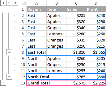
For example, this is how your Excel subtotals can look like:
How to insert subtotals in Excel
To quickly add subtotals in Excel, perform the following steps.
1. Organize the source data
The Excel Subtotal feature requires that the source data be arranged in a proper order and should not contain any blank rows.
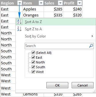
So, before adding subtotals, be sure to sort the column that you want to group your data by. The easiest way to do this, is click the Filter button on the Data tab, then click the filter arrow, and select to sort either A to Z or Z to A:
To remove blank cells without messing up your data, please follow these guidelines: How to remove all blank rows in Excel.
2. Add subtotals
Select any cell within your dataset, go to the Data tab > Outline group, and click Subtotal.

Tip. If you want to add subtotals only for some part of your data, select the desired range before clicking the Subtotal button.
3. Define the subtotal options
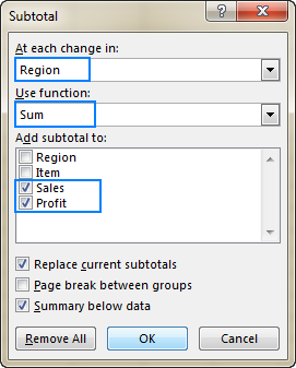
In the Subtotal dialog box, specify the three primary things - which column to group by, what summary function to use, and which columns to subtotal:
- In the At each change in box, select the column containing the data that you want to group by.
- In the Use function box, select one of the following functions:
- Sum - add up the numbers.
- Count - count non-empty cells (this will insert Subtotal formulas with the COUNTA function).
- Average - calculate the average of numbers.
- Max - return the largest value.
- Min - return the smallest value.
- Product - calculate the product of cells.
- Count Numbers - count cells that contain numbers (this will insert Subtotal formulas with the COUNT function).
- StdDev - calculate the standard deviation of a population based on a sample of numbers.
- StdDevp - return the standard deviation based on an entire population of numbers.
- Var - estimate the variance of a population based on a sample of numbers.
- Varp - estimate the variance of a population based on an entire population of numbers.
- Under Add subtotal to, select the check box for each column that you want to subtotal.
In this example, we group the data by the Region column, and use the SUM function to total numbers in the Sales and Profit columns.
Additionally, you can select any of the following option:
- To insert an automatic page break after each subtotal, select the Page break between groups box.
- To display a summary row above the details row, clear the Summary below data box. To show a summary row below the details row, select this check box (usually selected by default).
- To overwrite any existing subtotals, keep the Replace current subtotals box selected, otherwise clear this box.
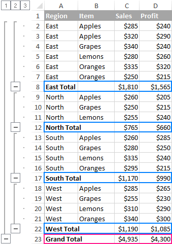
Finally, click the OK button. The subtotals will appear below each data group, and the grand total will be added to the end of the table.
Once subtotals are inserted in your worksheet, they will recalculate automatically as you edit the source data.
Tip. If the subtotals and grand total are not recalculated, be sure to set your workbook to automatically calculate formulas (File > Options> Formulas > Calculation options > Workbook Calculation > Automatic).
3 things you should know about Excel Subtotal feature
Excel Subtotal is very powerful and versatile, and at the same time it's a very specific feature in terms of how it calculates data. Below, you will find the detailed explanations of Subtotal's specificities.
1. Only visible rows are subtotaled
In essence, Excel Subtotal calculates values in visible cells and ignores filtered out rows. However, it includes values in rows hidden manually, i.e. the rows that were hidden by using the Hide Rows command on the Home tab > Cells group > Format > Hide & Unhide, or by right clicking the rows, and then clicking Hide. The following few paragraphs explain the technicalities.
Applying the Subtotal feature in Excel automatically creates SUBTOTAL formulas that perform a specific calculation type such as sum, count, average, etc. The function is defined by the number in the first argument (function_num) that belongs to one of the following sets:
- 1 - 11 ignore filtered-out cells, but include manually hidden rows.
- 101 - 111 ignore all hidden rows (filtered out and hidden manually).
The Excel Subtotal feature inserts formulas with function number 1-11.
In the above example, inserting subtotals with the Sum function creates this formula: SUBTOTAL(9, C2:C5). Where 9 represents the SUM function, and C2:C5 is the first group of cells to subtotal.
If you filter out, say, Lemons and Oranges, they will be automatically removed from the subtotals. However, if you hide those rows manually, they will be included in the subtotals. The image below illustrates the difference:

To exclude manually hidden rows so that only visible cells are calculated, modify the Subtotal formula by replacing the function number 1-11 with the corresponding number 101-111.
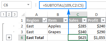
In our example, to sum only visible cells excluding manually hidden rows, change SUBTOTAL(9,C2:C5) to SUBTOTAL(109,C2:C5):
For more information about using Subtotal formulas in Excel, please check out the SUBTOTAL function tutorial.
2. Grand totals are calculated from the original data
The Excel Subtotal feature calculates grand totals from the original data, not from the subtotal values.
For example, inserting subtotals with the Average function calculates the Grand Average as an arithmetic mean of all original values in cells C2:C19, neglecting the values in the subtotal rows. Just compare the following screenshots to see the difference:

3. Subtotals are not available in Excel tables
If the Subtotal button is grayed out on your ribbon, then most likely you are working with an Excel table. Since the Subtotal feature cannot be used with Excel tables, you would need to convert your table to an ordinary range first. Please check out this tutorial for the detailed steps: How to convert Excel table to range.
How to add multiple subtotals in Excel (nested subtotals)
The previous example demonstrated how to insert one level of subtotals. And now, let's take it further and add subtotals for inner groups within the corresponding outer groups. More specifically, we will group our sample data by Region first, and then break it down by Item.
1. Sort data by several columns
When inserting nested subtotals in Excel, it is important that you sort the data in all the columns that you want to group your subtotals by. To do this, go to the Data tab > Sort & Filter group, click the Sort button, and add two or more sorting levels:
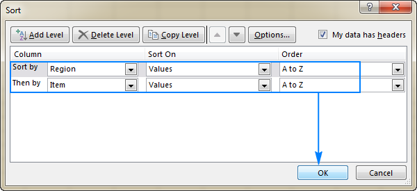
For the detailed instructions, please see How to sort by several columns.
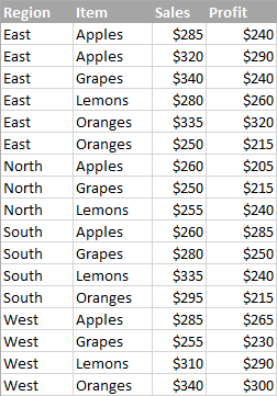
As the result, the values in the first two columns are sorted in alphabetical order:
2. Insert the first level of subtotals
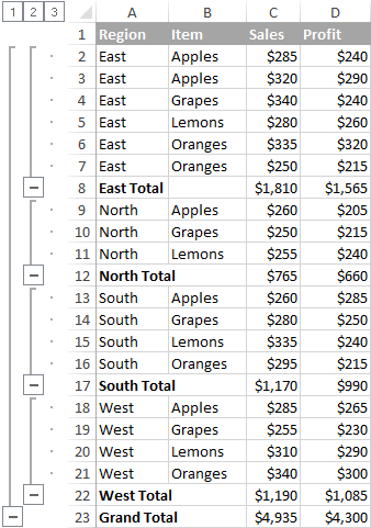
Select any cell within your data list, and add the first, outer level, of subtotals as demonstrated in the previous example. As the result, you will have Sales and Profit subtotals per Region:
3. Insert nested levels of subtotals
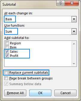
With the outer subtotals in place, click Data > Subtotals again to add an inner subtotal level:
- In the At each change in box, select the second column you want to group your data by.
- In the Use function box, select the desired summary function.
- Under Add subtotal to, select the column(s) for which you want to calculate subtotals. This can be the same column(s) as in the outer subtotals or different ones.
Finally, clear the Replace current subtotals box. It is the key point that prevents overwriting the outer level of subtotals.
Repeat this step to add more nested subtotals, if needed.
In this example, the inner subtotal level will group data by the Item column, and sum up values in Sales and Profit columns:
As the result, Excel will calculate the totals for each item within each region, as shown in the below screenshot:
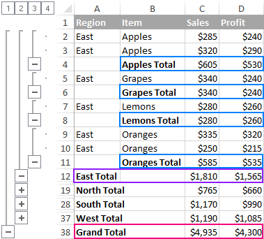
For the sake of room, the East Region group is expanded to display the nested Item subtotals, and 3 other region groups are collapsed (the following section explains how to do this: Display or hide subtotal details).
Add different subtotals for the same column
When using subtotals in Excel, you are not limited to inserting just one subtotal per column. In fact, you can summarize data in the same column with as many different functions as you want.
For example, in our sample table, in addition to Region totals we could display an average for the Sales and Profit columns:
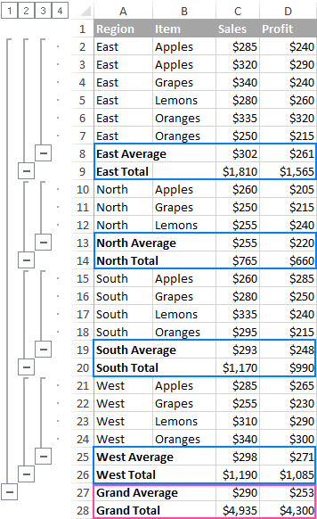
To get a result similar to what you see in the screenshot above, perform the steps described in How to add multiple subtotals in Excel. Just remember to clear the Replace current subtotals box every time you are adding the second and all subsequent levels of subtotals.
How to use subtotals in Excel
Now that you know how to do subtotals in Excel to instantly get a summary for different groups of data, the following tips will help you get the Excel Subtotal feature under your full control.
Show or hide subtotal details
To display the data summary, i.e. only subtotals and grand totals, click one of the outline symbols ![]() that appear in the upper-left corner of your worksheet:
that appear in the upper-left corner of your worksheet:
- Number 1 displays only the grand totals.
- The last number displays both subtotals and individual values.
- In-between numbers show groupings. Depending on how many subtotals you have inserted in your worksheet, there may be one, two, three or more in-between numbers in the outline.
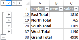
In our sample worksheet, click number 2 to display the first grouping by Region:
Or, click number 3 to display the nested subtotals by Item:
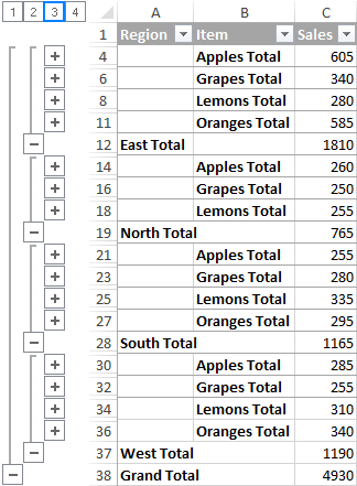
To display or hide data rows for individual subtotals, use the ![]() and
and ![]() symbols.
symbols.
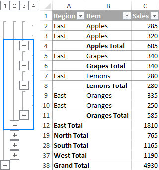
Or, click the Show Details and Hide Details buttons on the Data tab, in the Outline group.

Copy only subtotal rows
As you see, using Subtotal in Excel is easy… until it comes to copying only subtotals to somewhere else.
The most obvious way that comes to mind - display the desired subtotals, and then copy those rows to another location - won't work! Excel will copy and paste all of the rows, not only the visible rows included in the selection.
To copy just the visible rows containing subtotals, perform these steps:
- Display only the subtotal rows that you want to copy by using outline numbers or plus and minus symbols.
- Select any subtotal cell, and then press Ctrl+A to select all cells.
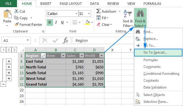
- With the subtotals selected, go to the Home tab > Editing group, and click Find & Select > Go to Special…
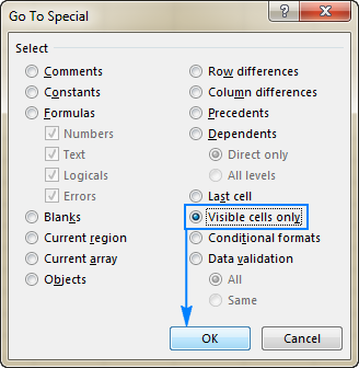
- In the Go To Special dialog box, select Visible Cells only, and click OK.
Tip. Instead of using the Go To Special feature, you can press Alt + ; to select only visible cells.
- In your current worksheet, press Ctrl+C to copy the selected subtotal cells.
- Open another sheet or workbook, and press Ctrl+V to paste the subtotals.
Done! As the result, you have just the data summary copied to another worksheet. Please note, this method copies the subtotal values and not the formulas:
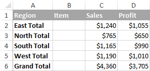
Tip. You can use the same trick to change the formatting of all subtotal rows in one fell swoop.
How to change subtotals
To quickly modify the existing subtotals, just do the following:
- Select any subtotal cell.
- Go to the Data tab, and click Subtotal.
- In the Subtotal dialog box, make any changes you want pertaining to the key column, summary function and values to be subtotaled.
- Make sure the Replace current subtotals box is selected.
- Click OK.
Note. If multiple subtotals were added for the same dataset, it's not possible to edit them. The only way is to remove all existing subtotals, and then insert them anew.
How to remove subtotals in Excel
To remove subtotals, follow these steps:
- Select any cell in the subtotals range.
- Go to the Data tab > Outline group, and click Subtotal.
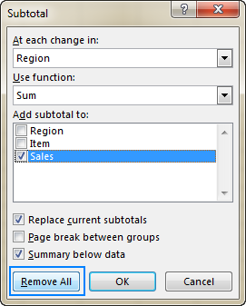
- In the Subtotal dialog box, click the Remove All button.
This will ungroup your data and delete all of the existing subtotals.
Apart from the Excel Subtotal feature that inserts subtotals automatically, there is a "manual" way to add subtotals in Excel - by using the SUBTOTAL function. It provides even more versatility, and the above linked tutorial shows a couple of useful tricks.
 by
by
19 comments
How to copy only visible cells (e.g. Subtotal Rows):
Press ALT + (colon) :
(All rows in concern should like light up)
CTRL C
CTRL V
How can I apply conditional format to highlight subtotals greater than a number?
My report has positive and negative subtotals and I want to highlight only subtotals greater than 19 and -19 please?
Hi! To color the rows with subtotals, use this instruction: Change the row color based on cell value. A conditional formatting formula might look something like this:
=AND(ISNUMBER(SEARCH("Total",$D1)), $E1>19)
I hope my advice will help you solve your task.
How to do subtotals in excel in different work sheet used in single formula.
I have a work breakdown structure in excel, complete with tasks, sub-tasks, sub-sub-tasks,... I group these accordingly (e.g. tasks are level 1, sub-tasks are level 2, etc.). I have a column with task numbers (e.g. 1, 1.1, 1.2, 1.2.1, 1.2.2, 2, etc.) and a second column with the task description. I then have subsequent columns for each resource where I enter the number of hours necessary to complete the lowest level task. I would like to get the roll-up of hours by resource for a particular level task level. Seems like a natural application of the SUBTOTAL function, but I do not have a column that specifies the level of the task on which to sort. Do I have to add a superfluous column with the specified level number to be able to do the subtotal, or can I somehow access the level directly from the grouping (Excel knows the level)?
Thank you in advance for any pointers or best practices.
Very Helpfull, thank you
how can register result of sum in another cell which after deleting reference values of sum it does not change i another word result remain even after deleting values
You have done a very great work. Thank you very much. This is very helpful.
I HAVE FOUR COLUMNS IN EXCEL 1. PARTY NAME 2. GST NO 3.VALUE 4. TAX WHEN I SUBTOTAL THE VALUE AND TAX IT SHOWS TOTAL OF THE BOTH. WHEN I SELECT SUB TOTAL OPTION NO 2 IT DISPLAY THE SUBTOTAL ROWS ONLY. BUT I NEED IN THIS FIELD GSST NO OF THE PARTY. IT NOT DISPLAY ITS SHOWS ONLY BLANK. HOW TO GET THE GST NO IN OPTION 2 IN SUBTOTAL
Great Help. Keep it up!
I have an excel sheet which contains four columns, date, description, name and amount.
I have entered all the data required but I got to the last amount in the last column and up came a Total figure. How do I get rid of that total and just enter the normal amount which should be there. Every time I type in $26-10 it goes to $46,600.00. This is so frustrating, I dont know much about excel. Thank you for any help. Maxine
I accidentally did something that appears to give me the option to subtotal (it has the 1-5 on the left and 1-7 on the top) How do I get rid of this if I don't want to see this since it is making my data screen so much smaller?
I'm trying to learn applying Subtotals in Excel 2010. However, the automatic Subtotal feature doesn't work for me. As soon as I select cells, it greys out (=inactive).
I have several columns:
Price / minus Discount / = Subtotal / plus Addl. Cost / = GRAND Total
How do I accomplish that?
Sounds as if your data is in a table. If so, Subtotals are not supported in Excel tables. The Subtotal command will appear grayed out if you are working with an Excel table. To add subtotals in a table, you must first convert the table to a normal range of data, and then add the subtotal. Note that this will remove all table functionality from the data except table formatting. Or you can create a PivotTable.
Hi
I got some hints from this article (nested levels of subtotals) and think it may help what I am trying to accomplish. But how do you copy other column data together with the subtotal data? For example in the source data, there could be a column 'Brand', indicating the brand of the fruits. I want to copy this column info to another worksheet:
East Apples BrandA 605
East Grapes BrandB 340
East Lemons BrandC 280
:
:
Can I do that? Note that all East Apples have same BrandA, all East Grapes have same BrandB.... The brand is just for reference purpose.
When i use subtotal to replace, existing column groupings getting ungrouped; How to retain column grouping while using subtotal multiple no. of times?
Saw the Above or Below for placement of the Subtotal.
In the process of automating dozens of reports with VBA.
The unique report uses both Above and Below.
A.K.A. Bracketed Subtotal Titles
e.g.
Area1
group1
group2
Area1 Subtotal
Area2
group1
group2
Area2 Subtotal
The idea is that in a collapsed view, it can be copied and pasted into a Power Point Presentation with formatting.
It appears that this will take vba to accomplish?
awesome. very helpful article. thanks a lot.
Hi...
Wow its a great blog ..
I dont have switch function in my excel desktop 2016...
Do i get a udf ..tried all over internet ....