The tutorial shows how to do subtraction in Excel by using the minus sign and SUM function. You will also learn how to subtract cells, entire columns, matrices and lists.
Subtraction is one of the four basic arithmetic operations, and every primary school pupil knows that to subtract one number from another you use the minus sign. This good old method works in Excel too. What kind of things can you subtract in your worksheets? Just any things: numbers, percentages, days, months, hours, minutes and seconds. You can even subtract matrices, text strings and lists. Now, let's take a look at how you can do all this.
Subtraction formula in Excel (minus formula)
For the sake of clarity, the SUBTRACT function in Excel does not exist. To perform a simple subtraction operation, you use the minus sign (-).
The basic Excel subtraction formula is as simple as this:
For example, to subtract 10 from 100, write the below equation and get 90 as the result:
=100-10
To enter the formula in your worksheet, do the following:
- In a cell where you want the result to appear, type the equality sign (=).
- Type the first number followed by the minus sign followed by the second number.
- Complete the formula by pressing the Enter key.
Like in math, you can perform more than one arithmetic operation within a single formula.
For example, to subtract a few numbers from 100, type all those numbers separated by a minus sign:
=100-10-20-30
To indicate which part of the formula should be calculated first, use parentheses. For example:
=(100-10)/(80-20)
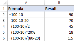
The screenshot below shows a few more formulas to subtract numbers in Excel:
How to subtract cells in Excel
To subtract one cell from another, you also use the minus formula but supply cell references instead of actual numbers:
For example, to subtract the number in B2 from the number in A2, use this formula:
=A2-B2
You do not necessarily have to type cell references manually, you can quickly add them to the formula by selecting the corresponding cells. Here's how:
- In the cell where you want to output the difference, type the equals sign (=) to begin your formula.
- Click on the cell containing a minuend (a number from which another number is to be subtracted). Its reference will be added to the formula automatically (A2).
- Type a minus sign (-).
- Click on the cell containing a subtrahend (a number to be subtracted) to add its reference to the formula (B2).
- Press the Enter key to complete your formula.
And you will have a result similar to this:

How to subtract multiple cells from one cell in Excel
To subtract multiple cells from the same cell, you can use any of the following methods.
Method 1. Minus sign
Simply type several cell references separated by a minus sign like we did when subtracting multiple numbers.
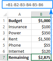
For example, to subtract cells B2:B6 from B1, construct a formula in this way:
=B1-B2-B3-B4-B5-B6
Method 2. SUM function
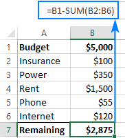
To make your formula more compact, add up the subtrahends (B2:B6) using the SUM function, and then subtract the sum from the minuend (B1):
=B1-SUM(B2:B6)
Method 3. Sum negative numbers
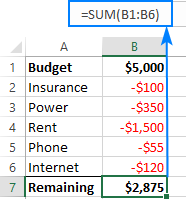
As you may remember from a math course, subtracting a negative number is the same as adding it. So, make all the numbers you want to subtract negative (for this, simply type a minus sign before a number), and then use the SUM function to add up the negative numbers:
=SUM(B1:B6)
How to subtract columns in Excel
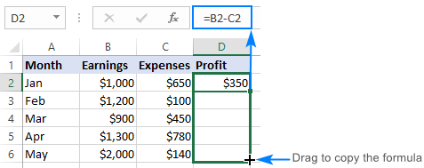
To subtract 2 columns row-by-row, write a minus formula for the topmost cell, and then drag the fill handle or double-click the plus sign to copy the formula to the entire column.
As an example, let's subtract numbers in column C from the numbers in column B, beginning with row 2:
=B2-C2
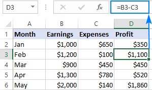
Due to the use of relative cell references, the formula will adjust properly for each row:
Subtract the same number from a column of numbers
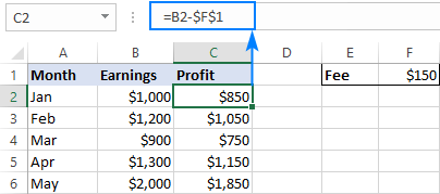
To subtract one number from a range of cells, enter that number in some cell (F1 in this example), and subtract cell F1 from the first cell in the range:
=B2-$F$1
The key point is to lock the reference for the cell to be subtracted with the $ sign. This creates an absolute cell reference that does not change no matter where the formula is copied. The first reference (B2) is not locked, so it changes for each row.
As the result, in cell C3 you will have the formula =B3-$F$1; in cell C4 the formula will change to =B4-$F$1, and so on:
If the design of your worksheet does not allow for an extra cell to accommodate the number to be subtracted, nothing prevents you from hardcoding it directly in the formula:
=B2-150
How to subtract percentage in Excel
If you want to simply subtract one percentage from another, the already familiar minus formula will work a treat. For example:
=100%-30%
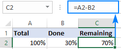
Or, you can enter the percentages in individual cells and subtract those cells:
=A2-B2
If you wish to subtract percentage from a number, i.e. decrease number by percentage, then use this formula:
For example, here's how you can reduce the number in A2 by 30%:
=A2*(1-30%)
Or you can enter the percentage in an individual cell (say, B2) and refer to that cell by using an absolute reference:
=A2*(1-$B$2)
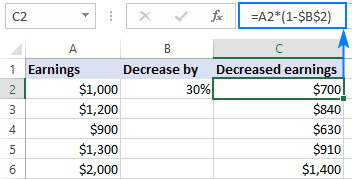
For more information, please see How to calculate percentage in Excel.
How to subtract dates in Excel
The easiest way to subtract dates in Excel is to enter them in individual cells, and subtract one cell from the other:
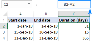
You can also supply dates directly in your formula with the help of the DATE or DATEVALUE function. For example:
=DATE(2018,2,1)-DATE(2018,1,1)
=DATEVALUE("2/1/2018")-DATEVALUE("1/1/2018")
More information about subtracting dates can be found here:
How to subtract time in Excel
The formula for subtracting time in Excel is built in a similar way:
For example, to get the difference between the times in A2 and B2, use this formula:
=A2-B2
For the result to display correctly, be sure to apply the Time format to the formula cell:
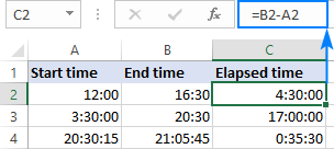
You can achieve the same result by supplying the time values directly in the formula. For Excel to understand the times correctly, use the TIMEVALUE function:
=TIMEVALUE("4:30 PM")-TIMEVALUE("12:00 PM")
For more information about subtracting times, please see:
How to do matrix subtraction in Excel
Suppose you have two sets of values (matrices) and you want to subtract the corresponding elements of the sets like shown in the screenshot below:
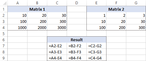
Here's how you can do this with a single formula:
- Select a range of empty cells that has the same number of rows and columns as your matrices.
- In the selected range or in the formula bar, type the matrix subtraction formula:
=(A2:C4)-(E2:G4) - Press Ctrl + Shift + Enter to make it an array formula.
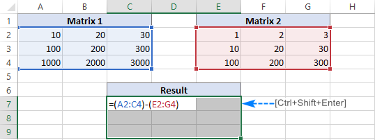
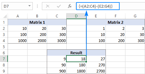
The results of the subtraction will appear in the selected range. If you click on any cell in the resulting array and look at the formula bar, you will see that the formula is surrounded by {curly braces}, which is a visual indication of array formulas in Excel:
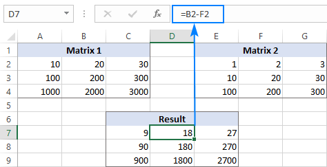
If you do not like using array formulas in your worksheets, then you can insert a normal subtraction formula in the top leftmost cell and copy in rightwards and downwards to as many cells as your matrices have rows and columns.
In this example, we could put the below formula in C7 and drag it to the next 2 columns and 2 rows:
=A2-C4
Due to the use of relative cell references (without the $ sign), the formula will adjust based on a relative position of the column and row where it is copied:
Subtract text of one cell from another cell
Depending on whether you want to treat the uppercase and lowercase characters as the same or different, use one of the following formulas.
Case-sensitive formula to subtract text
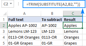
To subtract text of one cell from the text in another cell, use the SUBSTITUTE function to replace the text to be subtracted with an empty string, and then TRIM extra spaces:
With the full text in A2 and substring you want to remove in B2, the formula goes as follows:
=TRIM(SUBSTITUTE(A2,B2,""))
As you can see, the formula works beautifully for subtracting a substring from the beginning and from the end of a string:
If you want to subtract the same text from a range of cells, you can "hard-code" that text in your formula.
As an example, let's remove the word "Apples" from cell A2:
=TRIM(SUBSTITUTE(A2,"Apples",""))
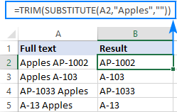
For the formula to work, please be sure to type the text exactly, including the character case.
Case-insensitive formula to subtract text
This formula is based on the same approach - replacing the text to subtract with an empty string. But this time, we will be using the REPLACE function in combination with two other functions that determine where to start and how many characters to replace:
- The SEARCH function returns the position of the first character to subtract within the original string, ignoring text case. This number goes to the start_num argument of the REPLACE function.
- The LEN function finds the length of a substring that should be removed. This number goes to the num_chars argument of REPLACE.
The complete formula looks as follows:
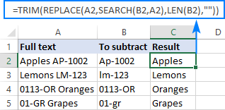
Applied to our sample data set, it takes the following shape:
=TRIM(REPLACE(A2,SEARCH(B2,A2),LEN(B2),""))
Where A2 is the original text and B2 is the substring to be removed.
Subtract one list from another
Supposing, you have two lists of text values in different columns, a smaller list being a subset of a larger list. The question is: How do you remove elements of the smaller list from the larger list?
Mathematically, the task boils down to subtracting the smaller list from the larger list:
Larger list: {"A", "B", "C", "D"}
Smaller list: {"A", "C"}
Result: {"B", "D"}
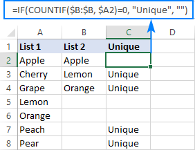
In terms of Excel, we need to compare two lists for unique values, i.e. find the values that appear only in the larger list. For this, use the formula explained in How to compare two columns for differences:
=IF(COUNTIF($B:$B, $A2)=0, "Unique", "")
Where A2 is the first cells of the larger list and B is the column accommodating the smaller list.
As the result, the unique values in the larger list are labeled accordingly:
And now, you can filter the unique values and copy them wherever you want.
That's how you subtract numbers and cells in Excel. To have a closer look at our examples, please feel free to download our sample workbook below. I thank you for reading and hope to see you on our blog next week!
Practice workbook
Subtraction formula examples (.xlsx file)
 by
by
99 comments
Create a formula that will subtract the value of D1 which is 22 from the value of A1 which is 12.
Hi!
The answer is in the first paragraph of this article.
How do you write a formula in excel which compares 4 numbers in 4 particular cells in order to determine the lowest number. Then subtract this lowest number from itself to arrive at 0 and also from the other 3 numbers in the 3 other cells to arrive at a new number.
Say the lowest number of the 4 numbers was 8 and the other 3 numbers were 12, 16 & 20. Then when a formula is inserted to compare those numbers the answers would automatically be 0, 4, 8 & 12.
Hello!
To find the minimum number in a range, use the MIN function:
=(A1:A4)-MIN(A1:A4)
Okay thanks
Hello,
I am working on an employee timesheet where they inform the hours worked and if they were OFF.
The formula is simple to see the hours worked, but I am struggling with the text (OFF) as I am getting the #VALUE! error.
Example: Start(C4) 8:00 / Finish (D4) 12:00 / Break(E4) 0:30 = (Finish - Start - Break)*24 = 3.50h
My problem is when they are OFF part time or full time. I have found the formula below that worked when they are all day OFF = showing 0h. But doesn't work when they inform hours.
=IF(ISERROR(D4*1),0,D4)-IF(ISERROR(C4*1),0,C4-IF(ISERROR(E4*1),0,E4))*24
Any help will be great, thank you in advance.
KR,
Graziella
Hi!
If "off" is written in cell D4, then you get a negative time, which is impossible. If there is a start time, then there must be an end time.
Thank you Alexander. Yes we always have the 3 information : start, finish and break. Is there any formula that understand the text as ZERO so and work correctly when there are hours as well?
Right now I do manually but really want to find something more easier.
Hi!
Your formula will convert text to zero. But if you write the end time "off", you will always get an error. You will subtract the start time from zero. I don't understand how the end time can be "off". What result do you want to get? Give an example of the source data and the expected result.
I also recommend reading this article: Calculate time in Excel: time difference, add, subtract and sum times.
Hello,
I've been trying to work this out for a while. So for example I want to 100-10, which equal 90. Then from that 90 get 40% which is 36. This should then be 54. However, I cannot seem to find a formula that works for me.
Thanks in advance!
Hi!
It's just simple math. =(100-10)*40%. or (100-10)*(100%-40%). Your explanations are not very clear. The following tutorial should help: How to do calculations in Excel.
Sorry! And thank you for that!
How to calculate (A%-B%) in excal
I have a column let be column B and i want to subtract B2-B1 and place it in E1, then in E2 i want B3-B2
and so on .so is there any function or formula that could help me ?
thank you .
Hi!
Formula in a cell E1: =B2-B1
Then copy the formula down the column as described in this guide: How to copy formula in Excel with or without changing references.
I had an old timer show me this formula many years ago, and now I'm the old timer who needs to use it again, but can't figure it out. I need to subtract Col. C from Col. D, and if the answer is a positive number it needs to go in Col. F, but if it is a negative number it needs to go in Col. E. This is for a surveying solution where the numbers in Col. C and D will always be different and the greater and lesser values of those columns can be in either of those columns. I hope that is clear, thank you very much.
Hi!
Use IF function in your formula:
in cell F1 =IF(D1 > C1,D1-C1,"")
in cell E1 =IF(C1 > D1,D1-C1,"")
Hope this is what you need.
=((B16/B24)*(1-B24)*12) I want to achieve
(B16/ B24) and (1-B24 ) multiply brackets and result to be multiplied by 12
Hi!
Parentheses are incorrectly placed in your formula
=((B16/B24)*(1-B24))*12
Hello, I’m trying to see if anyone knows if there is a way to subtract 2 values automatically every month. For example if I have 50 in a cell and I want to subtract 2 from 50 once a month how would I go about doing that?
Thanks
Hi,
I need formula for subtracting number from last cell, If my Column A have 20 which is total days and Column B have 18 Days Column C have 10 Days Column D have 5 Days, I need to get result as Column D should be 0, Column C should be 0, Column B should be 13. Based on total Days needs to reduce Total A column from last Column D, then C and then B.
Kindly help if anyone knows.
How to do this in excel
-3000 -(3000)
Hi ,
Please assist me on this ..
1 error = -5 points from the total points.. how to do in Excel.. we require 2 error = -10 like that..
Thank you
Hello!
If I understand your task correctly, the following formula should work for you:
=B1-C1*5
B1 - total points, C1 - number of errors
The value in A1 is 7.72%; the value in J1 is 12.79% (which is derived from adding C1+E1+F1). In L1, I want to get the value of J1 (12.79%) less/minus A1 (7.72%). What should be the formula in L1?
Hi,
If I understand your task correctly, the following formula should work for you:
=J1-A1
Can you help me...I am doing a running balance for accounting for probate court.
Say I started with balance of 1000.
If column A is a withdrawals of 50. and
Column B is a deposit of 1000., how do I get Column C to have the balance?
Hello!
Please check out this article to learn how to do a running total in Excel.
I hope my advice will help you solve your task.
if c1 value is 102+405 and d1 value is 104+605 and in c2 is 105+400 and d2 is 103+735 and so on, So how to subtract formula in column E
I’m trying to subtract multiple cells (expenses) across the board- from a single cell in my total income cell. This seems impossible, because I have tried every formula I’ve found on 6 different websites on how to do this, each one is completely different- and this entire page is contradictory.
Hi,
Please describe your task in detail, I’ll try to suggest a solution.
This is what i am trying to do as well - If i have a total of $300 in cell A1 and i put in $10 in cell B1 what is the formula i would use so that A1 would now be $290. This is for a budget - if i'm starting with a total dollar amount available i want to track each time i pay out from that total until it hits $0.
Hi!
An Excel formula can change the value only in the cell that it is pasted in. If you need to change the content on cell A1 that has some value in it, you’ll need to use a VBA macro. You can learn more about running total in Excel in this article on our blog.
Please can someone assist if I want to subtract 2.5% from an amount
Hi,
I hope you have studied the recommendations in the tutorial above.
I kindly ask you to have a closer look at the following paragraph of the article above — How to subtract percentage in Excel
00-24 - 04-07 how to subtract this kind of timing in excel
Hi,
I’m sorry but your task is not entirely clear to me. Could you please describe it in more detail? What result do you want to get? Give an example of the source data and the expected result.
Thank you!
You are using terms I don't understand. I just need to know:
the formula to subtract row 23 from row 25 across ALL columns?
Hello!
To subtract each position of line 23 from line 25 use the formula
=A25-A23
Copy the formula to the right line by line.
If this is not what you wanted, please describe your problem in more detail.
Hi Svetlana,
Is it possible to subtract the number of highlighted cells from a value in another cell. In context - I want to have a formula for amount of leave days available in one cell and deduct the number of highlighted cells (that correspond to days leave taken) from this ie days available = 10 - (3 highlighted cells in January) = 7 days leave remaining. Essentially not actually deducting a value but deducting a number of cells with no values within them.
I hope this makes sense! Or maybe there is another way to do it?
Many Thanks
Becky
Hello
I have typed in exel sheet 1000 but shwing 10 why Please resolve
Thank you soooo much, you saved me a lot of work.
hey
i want to know if it is possible to Subtract same name columns like for example if i have 5 apples and every time i type apple, one apple Subtract from these main number and these main number is in separate column.
thanks
Hello!
I’m sorry but your task is not entirely clear to me. For me to be able to help you better, please describe your task in more detail. Please specify what you were trying to find, what formula you used and what problem or error occurred. Give an example of the source data and the expected result.
It’ll help me understand it better and find a solution for you.
Hi, Is there a way I can have a cell calcuate and keep a running total each week.
Examaple
I have 2 columns:
C4-(Units to be billed)A number will be entered in this column weekly and D4 (Units Used) to keep a running total of data entered in C4 each week.
So If I enter 4 in C4 .. it will calcuate 4 in D4 but the following week if I enter 6 in C4 it should populate in 10 in D4.
Any help would be greatly appreciated.
Hello Lisa!
Read this article - Excel Cumulative Sum. How to calculate running total
Hi I want to if it's possible that.. If a enter a value in a cell can it automatically subtract the value of a different cell.. E g
Cell A1 has 940.. I want to manually enter 10940 in cell A2 and then it automatically shows 10000 in a cellA2.. Is there a formula for this
Hello Andy!
Either a formula or a value can be written in an Excel cell. If you entered 10940, then you can change this cell either manually or using the VBA.
Hi there,
I have a bit of a special request. I am trying to work out if it's possible to create a formula with numbers inside the same cell.
A1: Order # (as a prefix) 0000 - 0000 (range of the orders number)
B1: Combine order value
C1: How many unique orders were made( 1002 - 1001 = 1 order)
Example:
A1 B1 C1
Order # 1001 - 1002 Tot $ of the combined orders Numbers of unique orders
If A1 was divided in 2 cells it would be easy to do. In my case I was hoping to keep the orders numbers in the same cell.
Any idea if there is a formula so that I can extract the numbers after the "-" and subtract them with the numbers before the "-".
Thank you in advance.
Hi Svetlana
I hope this find you well
I am trying to find a formula to subtract the first 6 digits from a large string of digits, from one cell to another across column A and B
column A Column B
1234567891011122 123456
1234567891011122
1234567891011122
1234567891011122
many thanks
Amanda
Hello Amanda!
If the result should be a number, then use the formula
=--LEFT(TEXT(A1,"####"),6)
I hope this will help, otherwise please do not hesitate to contact me anytime.
Greetings....
Is it possible to subtract a number in a cell that is created by a formula? Example: Cell D43 has manually inputted number of 53.99, Cell D44 has a number of -4.00 which is the product of this formula =IF(D43=45.99;"-3.24";IF(D43=47.99;"-3.24";IF(D43=53.99;"-4.00";IF(D43=63.99;"-3.25"))))
Hello
lets say i have column with salaries that sums up at the end of the column is it possible to subtract a cell by highlighting it with color >>> so when the cell is highlighted the the number is subtracted from the total
thanks
Hello,
I need to create a formula to calculate shift times, column A is start time, column B is finish time but it goes over to the next day and excel does not recognise this when substracting =B1-A1.
What can I do?
Thank you
Hello,
I am attempting to create a formula that gives a value based of a range of cells when a new cell has data entered into. For example, i have set value in B1. When data is entered in C1, then i need the formula to =C1-B1. When data is entered in D1, then the formula should generate a value from D1-B1. And so on. Is this possible?
Hello. Can you tell me the formula if i want to subtract 1gram for each 10gram. For example if i punch in 79 in a cell in another cell it will be 72. And if i punch in 50 it will be 45. Your help would be appreciated thx
Lot of thanks team ablebits.com. This forum is fantastic. Your help is beyond words
Best regards
AK.
good work!
I’m trying to make a formula or command that if there is an actual number imputed in a specific cell then subtract the next actual imputed number from above in the same column. The numbers won’t be put in in the same cells all the time in that column. Example
1 2 3 4
A
B 300
C
D 600. I want cell D2 to take D1 and subtract it from
B1. But the formula needs to know that the 300 could have been in c1 or a1. I Want this to set up over 31 rows
Thank you so much!!
Hi. i'm mic. I have designed a box on a worksheet and includes letters From (A) to (Y) in columns B up to L out of 12 rows. The whole column A is where I input my data entry to receive results in this box. ie Column B has (5) edited bold letters from A to E. Skipping column C, column D has 5 letters from F to J. And skipping column E, column F has 5 letters from K to O. And this continues up to the last letter Y in column J. E.g Capital letter (A) is in column B2:3, letter (B) is in column B4:5, letter (C) is in column B6:7, and this continues up to (E) of column B. And this is also true to all the letters in the given columns. These letters represent the names of items that begin with these letters. And going to the cells of skipped columns, its where I receive the sum of each letter's existence in column A after an input. For example, letter (A) in column B has 2 cells, c2 and c3 in column C, and c3 (which is the down cell) is to give me the sum of A's appearance after its entry in column A. And here, all the down cells of the skipped columns are to give me the sum of each letters appearance in column A, and here I already used the COUNTIF function to do that for me. WHAT I WANT you to do for me is this. Lets say most letters in this box have different sums of entry from column A in their down cells, and in this case letter G has the sum of 6 entries in its down sum cell, yet G is the next entry but has not been entered in columm A since the last 13 entries. After its entry, how can I use letter G's upper cell (column C5) to count 0(zero) whenever G is entered and again start counting from 1 to 100( or more) if a another letter in entered. Or if letter A has the sum of 0(zero) in its down cell(that is column C3) since 36 last entries of other letters in column A, let column C2 (the upper cell) count 36 as its last(or none) entry in column A, and RETURN counting to zero if A is entered. Let the upper cells in the skipped columns of each letter independently count(sum) the number of times they were last entered and RETURN counting from zero when they have been entered in column A. What formula should I use to do this. PLIZ I NEED YOUR HELP. THX.
ON HAND 1 2 3 4 5 6 7 8 9 10
430 20 100 100 200 70 10 10 100 100 100
COVERED COVERED COVERED COVERED ONLY 10 Not Covered Not Covered Not Covered Not Covered Not Covered
the following line shows how the formula needs to put the correct info see below
1 2 3 4 5 6 7 8 9 10
0 0 0 0 60 10 10 100 100 100
hi
Based on my HAND I can cover from week 1 to week 4 and 10 pcs for week 5 and the rest of the week wont cover
Can you please help me to get the correct funtion and formula to use on this task ? pLease help thanks
Hello,
I created a spreadsheet that will subtract my postal charges from the total amount I created in a purchase request. Example: The Purchase request amount is $3,000.00, which populates cell F5. the mailing charges are subtracted for each cell in column G, so in cell G5 I typed $5.22 and then the results are shown in column H, or in this case cell H5, which tells me my remaining balance is $2,994.78. I now want the remaining balances I see for each individual cell in column H to show up in column F so that I don't have to type it in each cell in column F each time I get the balance. For example I want the $2,994.78 I see in cell H5 to now show up in F6. Then I will have the $2,994.78 in F6 subtract the mailing charge in G6 and get the remaining balance in H6, which will then reflect in F7 and so on. Is there a way to make this work?
PLEASE SUGGEST THE FORMULA FOR SUBTRACTION RESTRICTION WITH A NUMBER, SUPPOSE IN A TABLE VARIOUS ROWS FOR SUBTRACTION ARE THERE, THE AMOUNT TO BE SUBTRACTED IF BECOMES MORE THAN A CERTAIN NUMBER, THEN ALSO THE CERTAIN NUMBER ONLY SHOULD BE SUBTRACTED NOT THAT MORE NUMBER.
How to perform subtraction of 3 billion (3,000,000,000) frm 2 Septillion (2,000,000,000,000,000,000,000,000)?
It wun give the correct answer as if the 3B has been ignored.
I need help could you teach me how can I take the bonus for 2142worked hours 1500 hours must subtract the remaining hour it cost 10$. can you show me what formula i should use to see the bonus? ASAP thanks
TEXT ME HERE FOR CLASSES
I need a formula in excel that will add and subtract accrued time but not allow total to go over 384?
Dear Sir,
I don't want to put in the value every time I want to subtract one particular number from that cell. I tried placing that number in one cell and click it with =a1-b1 but this when extended using the easy option it selects the next one so I don't get the value. I don't want to put it inside the formula every time, cause this will be entered by someone else, that value they put in should be subtracted from all without making them the use of the formula.
THIS IS VERY IMPORTANT FOR ME
THANK YOU
i have followed this to the letter... just trying to subtract one column from the other.... does not work.
Hi Dana,
You may want to download our sample workbook and see how the formula is implemented there. Hope that will be helpful.
I have a cell with the formula =DATEDIF(G7,C2,"d") to get the number of days since a breeding event for cattle. I would like to be able to have another cell that automatically subtracts that number from 282, changing each day (like a countdown of days left, where 282 is the total days in gestation so I know how many days until they are due).
Thank you!
Lindsay
Hi Lindsay,
How about using the Excel DAYS function instead of the DATEDIF one? If that is okay with you, the formula is as follows:
=282 - DAYS(TODAY(), G7)
Honestly, this is awesome! It was as if i was face-to-face in a classroom with my tutor. This is excel made simple. Thank you so much.
I have value in cell a1 (1801381), I need to multiple that value by 1.05% (1891450), then subtract the value in cell A1 (1801381) from 1891450. What would that formula look like?
subtract function does not exist in excel ???? but you write =c1-c2 let say. too me it looks like a function but it works only once why ?
Hi Bob,
Functions and formulas are a bit different things.
Function is a predefined formula already available in Excel. Functions perform specific calculations based on the specified values, called arguments, or parameters.
For example, Excel provides a built-in function to add up numbers: SUM(number1,[number2],...)
A built-in SUBTRACT function does not exist. But you can make your own subtract formula like =A1-A2
Hi,
I'm currently trying to write a function for a time sheet at work and am having a little bit of trouble. My goal is to alert my boss when a task is close to being due but i've run into a bump thats making me scratch my head a little.
C5= 193 (HOURS ALLOWED ON PROJECT) E5= 183 (HOURS ACCUMULATED)
IF(C5=E5-10,"10 Hours Left")))
Any help would be appreciated. Thanks
Cameron,
It's not really a formula but if you were to type the following, it'll give you results that I think you're looking for:
=IF(E5=183,"10 Hours Left","")
If you need more help on your spreadsheet let me know. Ann
Hi..
I have students list with Marks & Rank and i want to find 1-10 marks how many students and their ranks in Brackets
For Example
1-10 marks
10 students(1,2,3,4,5,6,7,8,9,10)Ranks