Comparing columns in Excel is something that we all do once in a while. Microsoft Excel offers a number of options to compare and match data, but most of them focus on searching in one column. In this tutorial, we will explore several techniques to compare two columns in Excel and find matches and differences between them.
How to compare 2 columns in Excel row-by-row
When you do data analysis in Excel, one of the most frequent tasks is comparing data in each individual row. This task can be done by using the IF function, as demonstrated in the following examples.
Example 1. Compare two columns for matches or differences in the same row
To compare two columns in Excel row-by-row, write a usual IF formula that compares the first two cells. Enter the formula in some other column in the same row, and then copy it down to other cells by dragging the fill handle (a small square in the bottom-right corner of the selected cell). As you do this, the cursor changes to the plus sign:
To find cells within the same row having the same content, A2 and B2 in this example, the formula is as follows: To find cells in the same row with different values, simply replace the equals sign with the non-equality sign (<>): And of course, nothing prevents you from finding both matches and differences with a single formula: Or The result may look similar to this:
As you see, the formula handles numbers, dates, times and text strings equally well. Tip. You can also compare two columns row-by-row using Excel Advanced Filter. Here is an example showing how to filter matches and differences between 2 columns.
Formula for matches
=IF(A2=B2,"Match","")
Formula for differences
=IF(A2<>B2,"No match","")
Matches and differences
=IF(A2=B2,"Match","No match")=IF(A2<>B2,"No match","Match")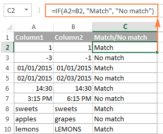
Example 2. Compare two lists for case-sensitive matches in the same row
As you have probably noticed, the formulas from the previous example ignore case when comparing text values, as in row 10 in the screenshot above. If you want to find case-sensitive matches between 2 columns in each row, then use the EXACT function:
=IF(EXACT(A2, B2), "Match", "")
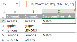
To find case-sensitive differences in the same row, enter the corresponding text ("Unique" in this example) in the 3rd argument of the IF function, e.g.:
=IF(EXACT(A2, B2), "Match", "Unique")
Compare multiple columns for matches in the same row
In your Excel worksheets, multiple columns can be compared based on the following criteria:
- Find rows with the same values in all columns (Example 1)
- Find rows with the same values in any 2 columns (Example 2)
Example 1. Find matches in all cells within the same row
If your table has three or more columns and you want to find rows that have the same values in all cells, an IF formula with an AND statement will work a treat:
=IF(AND(A2=B2, A2=C2), "Full match", "")
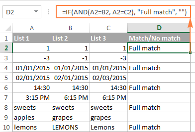
If your table has a lot of columns, a more elegant solution would be using the COUNTIF function:
=IF(COUNTIF($A2:$E2, $A2)=5, "Full match", "")
Where 5 is the number of columns you are comparing.
Example 2. Find matches in any two cells in the same row
If you are looking for a way to compare columns for any two or more cells with the same values within the same row, use an IF formula with an OR statement:
=IF(OR(A2=B2, B2=C2, A2=C2), "Match", "")
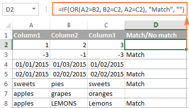
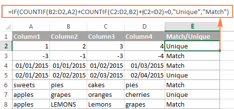
In case there are many columns to compare, your OR statement may grow too big in size. In this case, a better solution would be adding up several COUNTIF functions. The first COUNTIF counts how many columns have the same value as in the 1st column, the second COUNTIF counts how many of the remaining columns are equal to the 2nd column, and so on. If the count is 0, the formula returns "Unique", "Match" otherwise. For example:
=IF(COUNTIF(B2:D2,A2)+COUNTIF(C2:D2,B2)+(C2=D2)=0,"Unique","Match")
How to compare two columns in Excel for matches and differences
Suppose you have 2 lists of data in Excel, and you want to find all values (numbers, dates or text strings) which are in column A but not in column B.
For this, you can embed the COUNTIF($B:$B, $A2)=0 function in IF's logical test and check if it returns zero (no match is found) or any other number (at least 1 match is found).
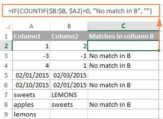
For instance, the following IF/COUNTIF formula searches across the entire column B for the value in cell A2. If no match is found, the formula returns "No match in B", an empty string otherwise:
=IF(COUNTIF($B:$B, $A2)=0, "No match in B", "")
Tip. If your table has a fixed number of rows, you can specify a certain range (e.g. $B2:$B10) rather than the entire column ($B:$B) for the formula to work faster on large data sets.
The same result can be achieved by using an IF formula with the embedded ISERROR and MATCH functions:
=IF(ISERROR(MATCH($A2,$B$2:$B$10,0)),"No match in B","")
Or, by using the following array formula (remember to press Ctrl + Shift + Enter to enter it correctly):
=IF(SUM(--($B$2:$B$10=$A2))=0, " No match in B", "")
If you want a single formula to identify both matches (duplicates) and differences (unique values), put some text for matches in the empty double quotes ("") in any of the above formulas. For example:
=IF(COUNTIF($B:$B, $A2)=0, "No match in B", "Match in B")
How to compare two lists in Excel and pull matches
Sometimes you may need not only match two columns in two different tables, but also pull matching entries from the lookup table. Microsoft Excel provides a special function for this - the VLOOKUP function. As an alternative, you can use a more powerful and versatile INDEX MATCH formula. The users of Excel 2021 and Excel 365, can accomplish the task with the XLOOKUP function.
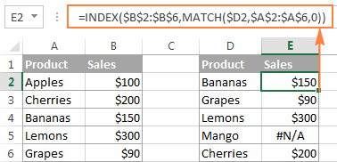
For example, the following formulas compare the product names in columns D against the names in column A and pull a corresponding sales figure from column B if a match is found, otherwise the #N/A error is returned.
=VLOOKUP(D2, $A$2:$B$6, 2, FALSE)
=INDEX($B$2:$B$6, MATCH($D2, $A$2:$A$6, 0))
=XLOOKUP(D2, $A$2:$A$6, $B$2:$B$6)
For more information, please see How to compare two columns using VLOOKUP.
If you don't feel very comfortable with formulas, you can have the job done using a fast and intuitive solution - Merge Tables Wizard.
Compare two lists and highlight matches and differences
When you compare columns in Excel, you may want to "visualize" the items that are present in one column but missing in the other. You can shade such cells in any color of your choosing by using the Excel Conditional Formatting feature and the following examples demonstrate the detailed steps.
Example 1. Highlight matches and differences in each row
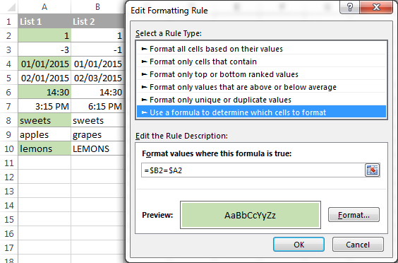
To compare two columns and Excel and highlight cells in column A that have identical entries in column B in the same row, do the following:
- Select the cells you want to highlight (you can select cells within one column or in several columns if you want to color entire rows).
- Click Conditional formatting > New Rule… > Use a formula to determine which cells to format.
- Create a rule with a simple formula like
=$B2=$A2(assuming that row 2 is the first row with data, not including the column header). Please double check that you use a relative row reference (without the $ sign) like in the formula above.
To highlight differences between column A and B, create a rule with this formula:
=$B2<>$A2
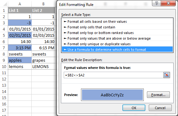
If you are new to Excel conditional formatting, please see How to create a formula-based conditional formatting rule for step-by-step instructions.
Example 2. Highlight unique entries in each list
Whenever you are comparing two lists in Excel, there are 3 item types that you can highlight:
- Items that are only in the 1st list (unique)
- Items that are only in the 2nd list (unique)
- Items that are in both lists (duplicates) - demonstrated in the next example.
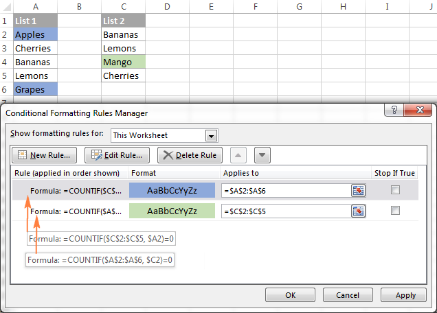
This example demonstrates how to color the items that are only in one list.
Supposing your List 1 is in column A (A2:A6) and List 2 in column C (C2:C5). You create the conditional formatting rules with the following formulas:
Highlight unique values in List 1 (column A):
=COUNTIF($C$2:$C$5, $A2)=0
Highlight unique values in List 2 (column C):
=COUNTIF($A$2:$A$6, $C2)=0
And get the following result:
Example 3. Highlight matches (duplicates) between 2 columns
If you closely followed the previous example, you won't have difficulties adjusting the COUNTIF formulas so that they find the matches rather than differences. All you have to do is to set the count greater than zero:
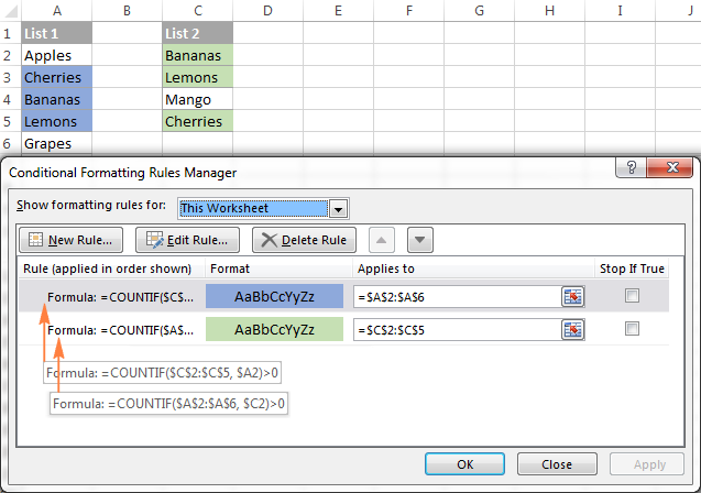
Highlight matches in List 1 (column A):
=COUNTIF($C$2:$C$5, $A2)>0
Highlight matches in List 2 (column C):
=COUNTIF($A$2:$A$6, $C2)>0
Highlight row differences and matches in multiple columns
When comparing values in several columns row-by-row, the quickest way to highlight matches is creating a conditional formatting rule, and the fastest way to shade differences is embracing the Go To Special feature, as demonstrated in the following examples.
Example 1. Compare multiple columns and highlight row matches
To highlight rows that have identical values in all columns, create a conditional formatting rule based on one of the following formulas:
=AND($A2=$B2, $A2=$C2)
or
=COUNTIF($A2:$C2, $A2)=3
Where A2, B2 and C2 are the top-most cells and 3 is the number of columns to compare.
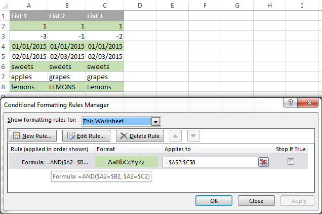
Of course, neither AND nor COUNTIF formula is limited to comparing only 3 columns, you can use similar formulas to highlight rows with the same values in 4, 5, 6 or more columns.
Example 2. Compare multiple columns and highlight row differences
To quickly highlight cells with different values in each individual row, you can use Excel's Go To Special feature.
- Select the range of cells you want to compare. In this example, I've selected cells A2 to C8.
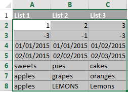
By default, the top-most cell of the selected range is the active cell, and the cells from the other selected columns in the same row will be compared to that cell. As you can see in the screenshot above, the active cell is white while all other cells of the selected range are highlighted. In this example, the active cell is A2, so the comparison column is column A.
To change the comparison column, use either the Tab key to navigate through selected cells from left to right, or the Enter key to move from top to bottom.
Tip. To select non-adjacent columns, select the first column, press and hold Ctrl, and then select the other columns. The active cell will be in the last column (or in the last block of adjacent columns). To change the comparison column, use the Tab or Enter key as described above.
- On the Home tab, go to Editing group, and click Find & Select > Go To Special… Then select Row differences and click the OK button.
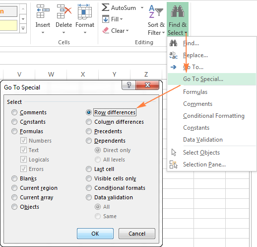
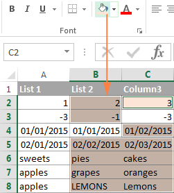
- The cells whose values are different from the comparison cell in each row are colored. If you want to shade the highlighted cells in some color, simply click the Fill Color icon on the ribbon and select the color of your choosing.
How to compare two cells in Excel
In fact, comparing 2 cells is a particular case of comparing two columns in Excel row-by-row except that you don't have to copy the formulas down to other cells in the column.
For example, to compare cells A1 and C1, you can use the following formulas.
For matches:
=IF(A1=C1, "Match", "")
For differences:
=IF(A1<>C1, "Difference", "")
To learn a few other ways to compare cells in Excel, please see:
Formula-free way to compare two columns / lists in Excel
Now that you know Excel's offerings for comparing and matching columns, let me show you our own solution for this task. This tool is named Compare Two Tables and it is included in our Ultimate Suite.
The add-in can compare two tables or lists by any number of columns and both identify matches/differences (as we did with formulas) and highlight them (as we did with conditional formatting).
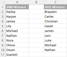
For the purpose of this article, we'll be comparing the following 2 lists to find common values that are present in both.
To compare two lists, here are the steps you need to follow:
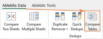
- Start with clicking the Compare Tables button on the Ablebits Data tab.
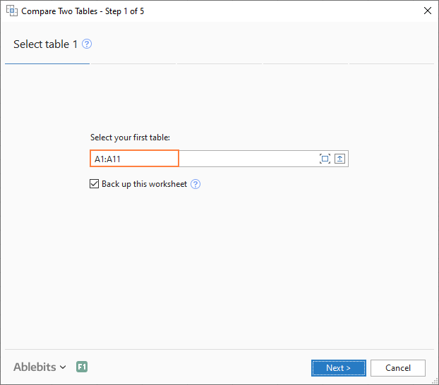
- Select the first column/list and click Next. In terms of the add-in, this is your Table 1.
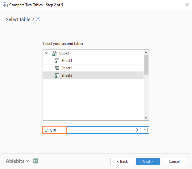
- Select the second column/list and click Next. In terms of the add-in, it is your Table 2, and it can reside in the same or different worksheet or even in another workbook.
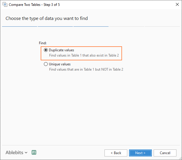
- Choose what kind of data to look for:
- Duplicate values (matches) - the items that exist in both lists.
- Unique values (differences) - the items that are present in list 1, but not in list 2.
Since our aim is to find matches, we select the first option and click Next.
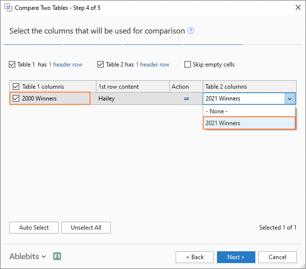
- This is the key step where you select the columns for comparison. In our case, the choice is obvious as we are only comparing 2 columns: 2000 Winners against 2021 Winners. In bigger tables, you can select several column pairs to compare by.
- In the final step, you choose how to deal with the found items and click Finish.
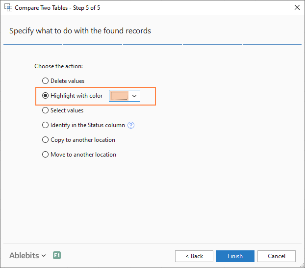
A few different options are available here. For our purposes, these two are most useful:
- Highlight with color - shades matches or differences in the selected color (like Excel conditional formatting does).
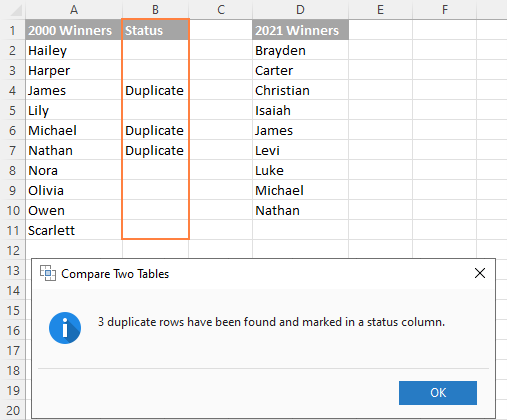
- Identify in the Status column - inserts the Status column with the "Duplicate" or "Unique" labels (like IF formulas do).
For this example, I've decided to highlight duplicates in the following color:
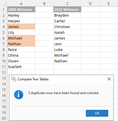
And in a moment, got the following result:
With the Status column, the result would look as follows:
Tip. If the lists you are comparing are in different worksheets or workbooks, it might be helpful to view Excel sheets side by side.
This is how you compare columns in Excel for matches (duplicates) and differences (unique values). If you are interested to try this tool, you are welcome to download an evaluation version using the below link.
I thank you for reading and encourage you to check out other helpful tutorials that we have :)
Available downloads
Compare Excel Lists - examples (.xlsx file)
Ultimate Suite - trial version (.exe file)
 by
by
548 comments
Hello I have a situation where i have column A with part number and column B which captures status if "quote recd" or "no quote".
the quotes are valid for 7 days. if i receive the same part number request on the 10th day i want to highlight that part number to check the status column and highlight if we have ever received quote for that part number.
i want to use conditional formatting to highlight that part number if anywhere in Column B it finds "quote recd".
Abbas:
Where are the dates stored? Wherever they are you can follow the same procedure to highlight them as outlined below.
If you want to highlight the B cell if it contains "Quote Recd" then select the cells that you want to highlight, go to Conditional Formatting, select the "Cells Equal To:", type Quote Recd" in the field and choose the formatting color of your choice. Click Save and then OK. Your cells should be filled with the formatting of your choice.
Thank you Svetlana Cheusheva. this article really helped me. keep up the great job.
Hello!
I have 2 different sheets. On sheet2, I want to find the PN 4324568 at what is the location and it pulls the data from sheet1 which is location 14. What formula do I need?
Sheet1
Col A
Row 1 PN 4324568
Row 2 Location 14
Sheet2
Col A
Row 1 PN 4324568
Row 2 Location ??
Thanks, Dan
Dan:
If you structure your data in sheet 1 by having PN in column A and their Location in column B you can do a VLOOKUP on sheet 2 like this:
In Sheet 2 column A enter the Part Numbers. In column B
directly across from the first part number enter
=VLOOKUP(A2,Sheet1!$A$2:$B$25,2,False) where A2 is the first part number for which you need a location and also
where Sheet1 A2:B25 are the cells which contain all of the part numbers and their locations.
Hi There,
I have an excel sheet with data in 3 different columns e.g F, H,I. I have to check the data present in col F is present in col H & I respectively. Is there any formula where I can check row by match.
I asked something similar in the countif section,but this may be a better place to ask. I'm looking just to get the number of matches between two columns when compared row by row. Is there any way to do this.
If I understand your question, this is how to get the sum of matches in two ranges of data:
=SUMPRODUCT(--(A39:A45=B39:B45))
Where A39:A45 is the first range of data and where B39:B45 is the second range of data.
So, this answers the question "What is the sum of the number of matches in these two ranges?" or put another way, "How many matches are there in this data?".
Hey, I want to compare 3 columns from one sheet to 3 columns in another sheet, can anybody help?
A B. C
2/3/18. 123
2/3/18. 123
1/3/18. 123
2/3/18. 124
I want a formula in C that return any text like say "ok" if B has multiple entry of same values and in A dates are different.
As in above 123 has 3 entries for these 3 entries column A has two dates 2/3/18 and 1/3/18, so formula should return OK as dates are different
Hi,
Below is a sample of the data I have. I want to match the data in Column A , B and C to data in Column F, G and H. If column A,B,C is not matching column F,G,H, I want to add a row and copy the data from Column A,B,C to F,G,H. For example, "880 0 1" is missing in column F,G,H, so I want to add a space and add "880 0 1" to column F,G,H so it will match column A,B,C. I have a large set of data, so I am trying to find a different way instead of checking for duplicate values in the two columns and manually adding one row at a time. Thanks!
A B C D E F G H
880 0 0 880 0 0
880 0 1 880 0 2
880 0 2 880 0 3
880 0 3 880 0 4
880 0 4
Hello,
Please I have one column and I need to know how to highlight two duplicated value but one (+) and one (-)
Ex.
123
142
-123
-142
Thank you!
Hello,
I have 2 lists
Column A has 1000 items in it
Colum B has 500 items in it
I'd like column C to be just a list of items that are NOT shared in either column A or B e.g. Let's say in the 1000 words in Column A - widget is there but no where in column B - I'd like the new list in column C to have the word widget in it along with all the others that are missing in the second column.
Hi, Please help with a formula with this:
I have 2 columns, one with a code (ex: XCSDADAS) and the other with URL embedded with a code. I need to compare both the columns to see if the code in column a matches with the code in the URL.
Thank you
I have 50separate bills of 50 customers in excel. I like to get each bill in another sheet with a reference at a click.Plz help me out.
Hi,
Thank you for helping in advance.
Please assist me in the following two columns, I need to compare two columns and extract the info like "AWC+ST" "AWC+BR" "RR+ST" "RR+BR" seperately.
Thanks & Regards.
Col1 Col2
RR ST
RR ST
RR ST
AWC ST
AWC ST
AWC ST
AWC ST
AWC ST
AWC ST
RR ST
AWC BR
AWC BR
AWC BR
RR BR
RR BR
AWC BR
AWC BR
AWC BR
AWC BR
AWC BR
RR BR
AWC BR
AWC BR
Hi Balaji,
I am sorry, it is not very clear what the result should look like. If you can send us a small sample workbook with your data and the result you want to get, we'll be able to help you better.
Please shorten your table to 10-20 rows / columns and email it to support@ablebits.com. Please also don't forget to include the link to your comment in the email.
Thank you.
I want to compare column A & B in list-1 with A & B In list-2.
I wont have duplicated data but list -1 it will not be in the the same order as list-2.
and some date may be missing from either list. after we compare A & B we need to compare A & C and so on
the files I want to compare to large file of data (I do this often),
I dont want to create a new helper table on the side its hard to keep organized
Can you just apply this idea directly to conditional formatting to spot differences?
I do not use VBA and they dont like VBA at work.
I have researched this to no avail.
I use Power query and power pivot if there is any help there
no one has a video on this
Thanks for your time
Kim Bilton
Hello. Please can you help me.
I have a to compare 2 sheets in the same workbook. One sheet has a full sheet of customer names (12000 rows), and the second has only a few (700). I need to check that the small sheet customers all exist in the big sheet, but there could be spelling mistakes or slight differences in writing customer names. For example, sheet 1 could have Toyota, and sheet 2 could have Toyota PTY.
How do I check the customer names, without scrolling through a 12000 row document.
Thanks.
I'm having a bit of a struggle. I have to columns. One contains the sales person's name and the other contains what they sold. I want to add the salesman's total to what type of product they sold. For example, sales person JW and the different products are home, pro, iLab. What formula can I use to give me a total number of sales for that particular item.
you saved me 72 hours of work in just a day. thnks
I have 3 excel columns which have values like this,
Col_A Col_B Col_C
----- ----- -----
400 600
500 800
400 300
300 200
700 900
800 700
500 100
I want the values to be copied in Column C from Column B, which are not Mache with Column A values.
I mean just copy the values from Column B, which are not available in Column A.
Like below
Col_C
-----
600
200
100
Is there any excel formula using which I can achieve this?
IF WE WANT TO MATCH TO 2 NO OF DIFFERENT COLUMN WITH AS SAME AS POSSIBLE DATA BUT NOT ACTUAL (EX- WB23B4152 IN (A) COLUMN BUT 4152 IN (B) COLUMN) THEN HOW WE CAN FIND?
Please help me
im in accounts and my bank statement didnt import correctly on to our system, i took the amounts from the bank into column b and the imported amouts in column A, what formula can i use to see what amount didnt import?
Hi (and Happy New Year), I would like to:
1)highlight cells with similar text (i.e: A1:blue and C12:Bluepoint) from two different columns
2)Count if and how many times a similar text in a cell (A1:Blue) appears in another cell of another column ((i.e: A1:blue, C12:Bluepoint and C25:Bluesky.
I have two columns with company names and I want to find duplicates (highlight them, count them), but the company names are not written always in the same way, i.e A1: cocacola ltd and C12: CocaCola company.
Is this possible?
Thanks a lot,Kos
New _Position code
JOB049130401803012001-002
JOB052110609801019002-004
JOB055350101805042003-005
JOB055350101805042003-006
JOB055350101805042003-007
JOB073850101805042003-004
JOB073850101805042003-005
JOB077910609801019002-003
JOB077912002801019002-001
JOB077912002801019002-0010
JOB077912002801019002-002
JOB077912002801019002-003
JOB077912002801019002-004
JOB077912002801019002-005
JOB077912002801019002-006
JOB077912002801019002-007
JOB077912002801019002-008
JOB077912002801019002-009
JOB078310107801019001-005
JOB080650101805222015-005
JOB086112001801039001-005
JOB086112001801039001-009
JOB086112001801039008-006
JOB086112001801039016-005
JOB086112001801039017-006
JOB086112001801039025-005
JOB086112001801039025-006
JOB090612002801152011-001
JOB090612002801152011-002
JOB090612002801152011-003
This is my list where i need to know which no is free to put in the end like -004,-005 etc which i have to put to create unique code. kinldy help me
JOB077912002801019002
Hello,
I'm afraid there's no easy way to solve your task with a formula. Using a VBA macro would be the best option here.
However, since we do not cover the programming area (VBA-related questions), I can advice you to try and look for the solution in VBA sections on mrexcel.com or excelforum.com.
Sorry I can't assist you better.
Hi
I want to know the excel formula to compare column E with A to D and get the mismatch indication at column F. Pl. help. Regards
A B C D E F
1 2 3 4 8
2 3 4 5 10
6 7 8 9 5
Hello,
For me to understand the problem better, please send me a small sample workbook with your source data and the result you expect to get to support@ablebits.com.
Please also don't forget to include the link to this comment into your email.
I'll look into your task and try to help.
May I ask how to pull out the text/string data different from column A (ie A2:A10) and Column B (B2:B10) to cloumn C
An example of raw data set:
A B C
Student Name: Student Name: Missing:
Tom Tom Jerry
Jerry Catherine Sam
Catherine Ada
Ada
Sam
Thank you!
Hello,
Please try the following formula:
=IFERROR(INDEX($A$2:$B$10,SMALL(IF(($B$2<>$A$2:$A$10)*($B$3<>$A$2:$A$10)*($B$4<>$A$2:$A$10)*($B$5<>$A$2:$A$10)*($B$6<>$A$2:$A$10)*($B$7<>$A$2:$A$10)*($B$8<>$A$2:$A$10)*($B$9<>$A$2:$A$10)*($B$10<>$A$2:$A$10),ROW($A$2:$A$10)-1),ROW(A1)),1),"")
Please note that this is an array formula. You should enter this formula into the first cell in column C, hit Ctrl + Shift + Enter to complete it and copy the formula down along the column. Just select the cell where you've entered the formula and drag the fill handle (a small square at the lower right-hand corner of the selected cell) down.
Hope it will help you.
I prefer to use Index/Match function instead of Vlookup. In Vlookup we can lookup values with [A5&"*"] option, which is not possible in the Match Function. Can I get a solution to use Index/Match Function with Match(A5&"*"] ?
WHEN I USE =$B2$C2 AS IN THE EXAMPLE ABOVE THERE IS NO RHYME OR REASON TO THE CELLS THAT ARE HIGHLIGHTED. COLUMNS THAT HAVE THE SAME VALUE ARE HIGHLIGHTED ALONG WITH SOME THAT ARE DIFFERNT LIKEWISE IF I USE = INSTEAD OF GET THE REVERSE OF THE CELL HIGHLIGHTE.
???????????????????????????????
Hello,
For me to understand the problem better, please send me a small sample workbook with your source data and the result you expect to get to support@ablebits.com. Please don't worry if you have confidential information there, we never disclose the data we get from our customers and delete it as soon as the problem is resolved.
Please also don't forget to include the link to this comment into your email.
I'll look into your task and try to help.
IF D2=D3 and A2 not equal to A3 insert the word "Duplicate hotkey" in column E
Sorry!
Hello,
For me to understand the problem better, please send me a small sample workbook with your source data and the result you expect to get to support@ablebits.com. Please don't worry if you have confidential information there, we never disclose the data we get from our customers and delete it as soon as the problem is resolved.
Please also don't forget to include the link to this comment into your email.
I'll look into your task and try to help.
IF D2=D3 and A2A3 insert the word "Duplicate hotkey" in column E
Hi Natalia,
Maybe you could help me with this formula?
I have a long Excel report of 37K lines that I would like to find duplicates in.
These duplicates should have different value in another column. So I thought maybe it will be possible to have a formula that will add a word next to these lines.
The formula needs to be along these lines (to my understanding):
IF D2=D3 and A2A3 insert the word "Duplicate hotkey" in column E
Would you be able to write such formula in Excel language?
Many thanks,
Avi
You just saved me so much time!!! Thank you!!!
I have received payment 100k
But In our books 200k with 300 invoice how i find matching invoices against 100k
i'm trying to track at what time of the day we have the biggest failure rate and highlight that time in the column. i have 5 columns, mon-fri. each column has rows broken into half hour increments. ex: row 4 is 8:30, row 5 is 9:00 etc. in the column in question, the value in row 4 is 10, row 5 is 19, row 6 is 27, row 7 is 31, row 8 is 60, and row 9 is 81. i can tell that the largest difference is between rows 7 & 8. is there a way to highlight row 8 to show that that is where the largest difference is? if so, how can i do it?
Thanks in advance.
A2- U 4 8 WENDLAND STREET PORT LINCOLN SA 5606
A3- U 1 5 SCANLAN STREET EAST BRISBANE QLD 4169
A4- U 16 7 BERYL STREET WESTMEAD NSW 2145
-----------------
B2- 4 8 WENDLAND STREET PORT LINCOLN SA 5606
B3- 8 HEIDELBERG STREET EAST BRISBANE QLD 4169
B4- 16 7 BERYL STREET WESTMEAD NSW 2145
When analyzing the differences in the above two data set. As you can see, A2 is similar to B2 (except for the letter U, which represents a Unit. For the purposes of my analysis, this is correct. As is A4 & B4). But clearly A3 is a different address to B3. How do i put a simple formulae in Except, which will extract the variations from two cells?
Thanks
Abs
How to compare 2 columns to find the match exist or not. I need the formula which compares B1 with A:A. If Match found 1 else 0. I tried =IF(B:B=AA, 1,0) didn't work.
A B
0001165186 0094713197
0001166595 0097094894
0001166619 0094640211
0001190181 0097058341
0001196342 0016685760
0001213475 0016748842
0001216979 0016760276
0001217648 0097012553
0001222292 0097075931
Hello, Sarah,
Please try this formula:
=IF(ISNA(VLOOKUP(B1,$A:$A,1,FALSE)),0,1)
Hello,
For work I am tasked with downloading customer Forecasts and updating our backlog accordingly. it is a very time consuming process. there are multiple parts that are on multiple different purchase orders with quantities and dates varying on a monthly basis. the changes are not that frequent but I have hundreds of rows to go through. I am looking for a way to quickly find changes that have occurred month to month however I need to hold reference to the part number, purchase order, quantity and date. have you any thoughts on how I may be able to do this?
Hello, William,
if I understand your task correctly, we have the add-in that may help you.
Please take a look at the Compare Two Tables tool from the Duplicate Remover add-in. With its help you'll be able to find unique records or remove duplicate values between 2 worksheets.
You can download a fully functional trial version to test the add-in and see if it work for you from this web-page:
https://www.ablebits.com/downloads/index.php
Hope this'll help!
thanks.....
Hi,
I have set of lab values in one column & reference range in another column. I want to highlight the lab values which are "Out of Range" & "Within he Range". Please let me know; how to do that.
Pl provide function in excel
Suppose data I column a and b
Name marks
C 9
D 14
E 20
Ans to be in column c and d
Name marks
E 20
D 14
C 9
Name marks
A 9
C 8
D 20
Result to be
Name marks
D 20
A 9
C 8
Pl provide function in office 2007
Hi,
How to lookup the value if the 2 cells having same value, excel is considering 1st cell but not considering 2nd cell(It should be considered)
Example all the 4 cells having the code of 7555(Attachment below) here some of the row having different values and some of the column having different values
For me it should be added and required in another sheet
Code A B C
7555 395
7555 77 343
7555 158 262
7555 210
Really amazing and simplifying the efforts.
Hi,
What I'm trying to do is highlight a row if there is any text found in cells in column E and column I.
So it would look something like:
IF text in Cell E
AND
Text in Cell I
Colour row red
There will always be text in the E column, so I only need the row to highlight if there is text found in the I column.
How do I go about doing this?
Thanks in advance :)
Hi
I want to compare Data in 2 columns A and B and want to highlight the different words only. Eg . my A1 CELL contain Apple, Sweets, good
B1 cell contains
Apple, sweets, pizza, car
In above two cells in A1 good is extra word which is not present in CELL B1. Where as Cell B1 contains words " Pizza, car "which are not present in excel so how to highlight only these different words
I have lot of Data
Hi, Sandy,
I’m afraid there’s no way to highlight only duplicate words in Excel. All the formulas and our add-ins will select or highlight the entire cell.
I can only advise you to ask around Mr.Excel forum in case they come up with some VBA code for you.
I wish I could assist you better.
Is there a way where we can identify
1. % similarity
2. between 2 columns
3. With strings as data.
Example:
Column A | Column B | Match
Cat is back | Dog is back | 33%
Superman | Spiderman | 0%
Compare to worksheets Sheet2 to Sheet1, find sheet2 match and then return data sheet1 from in 1st cell of this matched column.
2 work sheets
1st sheet contains A=data to return (1234) + B-H data to match 456,789,012
2nd sheet contains criteria to match - look for 456 then return A (1234)
hi, i need a formula to detect the values of the weight in a column and if it is more than the value then to add 7.50 but if it is less then the value to add 4.
so for example if the products weigh less than 0.4 then i need the cell to add 4 but if they weigh more than to add 7.5
hi
i have three unequal column and i want to extract unique cells for first column in compare with two another columns. how can i do it?
Thank you very much. Its working. worth full article!
Salaam everyone.
I have two excel columns each containing 63,000 values. I want to find out all the values where entries of column A are greater than those of column B. How can I do that?
Thanks in advance
Stay blessed.
Hello Fiaz,
You can enter the following formula in the first cell with data, say A1:
=IF(A1>B1, TRUE, "")
Then, copy the formula to the entire column. And after that sort or filter your dataset by the formula column.
I am working on aligning university rankings, as you can see the universities are ranked differently in 2008-2009. Is there a way to use excel to align the universities with corresponding rankings? There are hundreds of them for 12 years, so you can see it is mammoth task.
2008 2008 2009 2009
Sussex 26 cardifff 26
Cardiff 27 Sussex 27
Queen's 28 Reading 28
Reading 29 Sussex 29
Glasgow 30 Surrey 30
Birming 31 Strathclyde 31
Manches 32 Manche 32