You may think percentage calculations are useful only if you use them for work. But in reality, they help you in everyday life. Do you know how to tip properly? Is this discount a real deal? How much will you pay with this interest rate? Come find the answers to these and other similar questions in this article.
What is percentage
As you most likely already know, percent (or per cent) means one-hundredth part. It is marked by a special sign: %, and represents a part of the whole.
For example, your and your 4 friends are getting a birthday gift for another friend. It costs $250 and you're chipping in together. What percent of the total you're investing in the present?
This is how you usually calculate percents:
Let's see: you're giving away $50. 50/250*100 – and you get 20% of the gift cost.
However, Google Sheets makes the task simpler by calculating some parts for you. Below I'll show you those basic formulas that will help you get different results depending on your task, whether calculating percentage change, percentage of the total, etc.
How to calculate percentage in Google Sheets
This is how Google spreadsheet calculates percentage:
Unlike the previous formula, this one doesn't multiply anything by 100. And there's a good reason for that. Simply set the format of cells to percent and Google Sheets will do the rest.
So how will this work on your data? Imagine you keep track of ordered and delivered fruits (columns B and C respectively). To calculate the percentage of what's been received, do the following:
- Enter the below formula to D2:
=C2/B2 - Copy it down your table.
-
Go to Format > Number > Percent in Google Sheets menu to apply the percentage view.
Note. You'll need to go over these steps to create any percentage formula in Google Sheets.
Tip. You can decrease and increase decimal places if necessary using the options from the Google toolbar:

Here's how the result looks on real data:
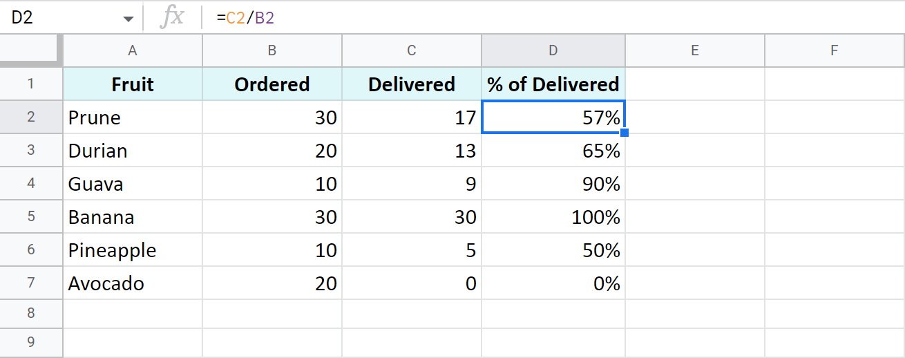
I removed all decimal places making the formula show the result as a rounded percent.
Percentage of a total in a Google spreadsheet
Here are a few more examples of calculating percentage of a total. Though the previous shows the same, it works great for that example but may not be enough for other data set. Let's see what else Google Sheets offers.
A common table with a total at its end
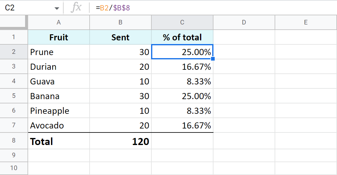
I believe this is the most common case: you have a table with values in column B. Their total resides at the very end of the data: B8. To find the percentage of the total for each fruit, use the same basic formula as before but with a slight difference – an absolute reference to the cell with the total sum.
This type of reference (absolute, with a dollar sign) doesn't change when you copy the formula to other cells. Thus, each new record will be calculated based on the sum in $B$8:
=B2/$B$8
I also formatted the results as percent and left 2 decimals to display:
One item takes a few rows – all rows are part of the total
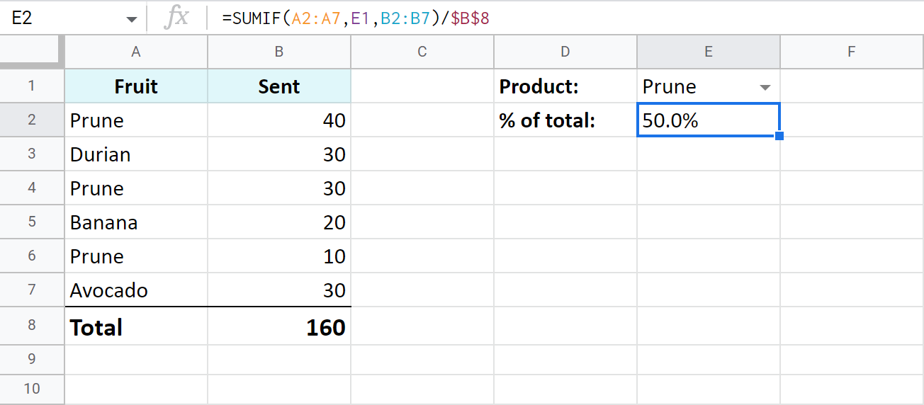
Now, suppose a fruit appears more than once in your table. What part of the total is composed of all deliveries of that fruit? The SUMIF function will help answer that:
It will sum only numbers belonging to the fruit of interest and divide the result by the total.
See for yourself: column A contains fruits, column B – orders for each fruit, B8 – the total of all orders. E1 has a drop-down list with all possible fruits where I chose to check the total for Prune. Here's the formula for this case:
=SUMIF(A2:A7,E1,B2:B7)/$B$8
Tip. Having a drop-down with fruits is completely up to you. Instead, you can put the necessary name right to the formula:
=SUMIF(A2:A7,"Prune",B2:B7)/$B$8
Tip. You can also check a part of the total made by different fruits. Just add up a few SUMIF functions and divide their result by the total:
=(SUMIF(A2:A7,"prune",B2:B7)+SUMIF(A2:A7,"durian",B2:B7))/$B$8
Percentage increase and decrease formulas
There's a standard formula you can use to calculate percent change in Google Sheets:
=(B-A)/A
The trick is to figure out which of your values belong to A and to B.
Let's assume you had $50 yesterday. You have saved $20 more and today you have $70. This is 40% more (increase). If, on the contrary, you've spent $20 and have only $30 left, this is 40% less (decrease). This deciphers the formula above and makes it clear which values should be used as A or B:
Let's see how this works in Google Sheets now, shall we?
Work out percent change from column to column
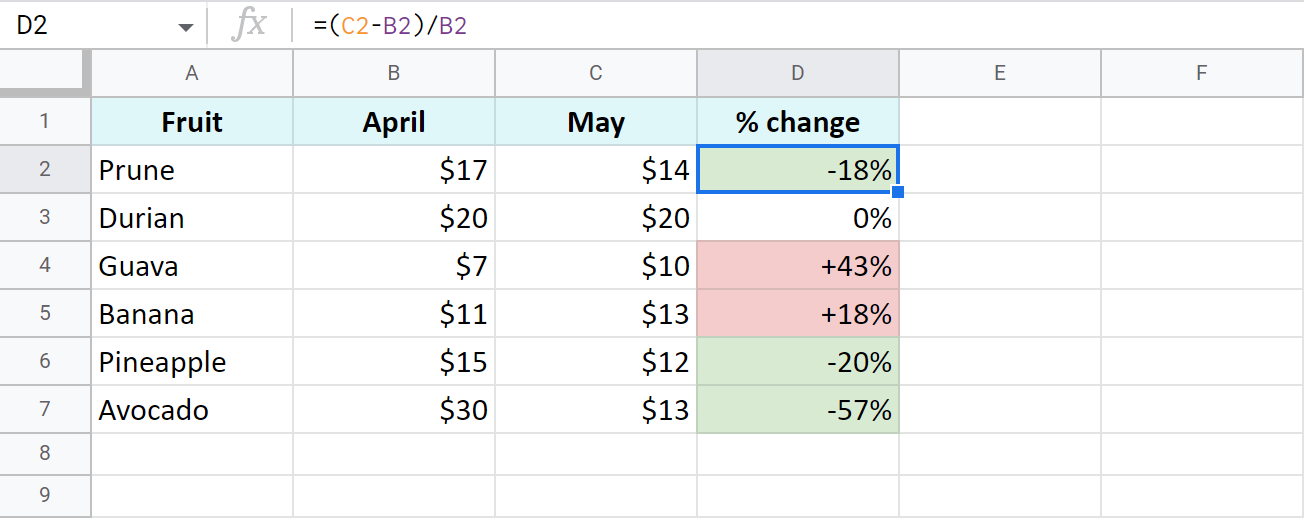
I have a list of fruits (column A) and I want to check how prices have shifted in this month (column C) compared to the previous one (columns B). Here's the percent change formula I use in Google Sheets:
=(C2-B2)/B2
Tip. Don't forget to apply the percent format and adjust the number of decimal places.
I also used conditional formatting to highlight cells with percent increase with red and percent decrease with green:
Percent change from row to row
This time, I'm tracking total sales (column B) over each month (column A). To make sure my formula works correctly, I should start entering it from the second row of my table – C3:
=(B3-B2)/B2
Copy the formula over all rows with data, apply the percent format, decide on the number of decimals, and voila:
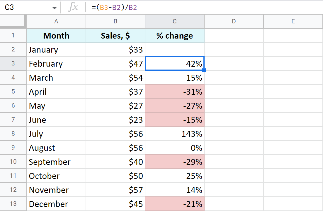
Here I also coloured percentage decrease with red.
Percent change compared to one cell
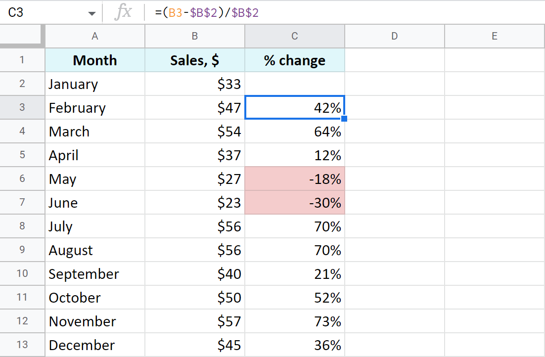
If you take the same sales list and decide to calculate percentage change based on January only, you will have to always refer to the same cell – B2. For that, make the reference to this cell absolute instead of relative so it doesn't change after copying the formula to other cells:
=(B3-$B$2)/$B$2
Amount and total by percentage in Google spreadsheets
Now that you've learned how to operate percentages, I hope getting total and the amount will be a child's play.
Find amount when having total and percentage
Let's imagine you've spent $450 shopping abroad and you'd like to have the taxes returned – 20%. So how much exactly should you expect to receive back? How much is 20% of $450? Here's how you should count:
If you put the total to A2 and the percent to B2, the formula for you is:
=A2*B2

Find total if you know amount and percentage
Another example: you've found an ad where a used scooter is being sold for $1,500. The price already includes a pleasant 40% discount. But how much would you need to pay for a new scooter like that? The below formula will do the trick:
As the discount is 40%, it means you are to pay 60% (100% – 40%). With these numbers at hand, you can work out the original price (total):
=A2/C2

Tip. As Google Sheets stores 60% as one hundredth – 0.6, you can get the same result with these two formulas as well:
=A2/0.6
=A2/60%
Increase and decrease numbers by percentage
The following examples represent the formulas you may need a bit more often than other ones.
Increase a number in a cell by percent
A general formula to calculate the raise by some percent is as follows:
If you have some amount in A2 and you need to increase it by 10% in B2, here's your formula:
=A2*(1+B2)

Decrease a number in a cell by percent
To make the opposite and decrease the number by a percent, use the same formula as above but replace the plus sign with a minus:
=A2*(1-B2)

Increase and decrease a whole column by percent
Now assume you have lots of records written in a column. You need to raise each of them by a percentage in that same column. There's a quick way (6 steps to be exact) to do that with our Power Tools add-on:
- Select all values you'd like to raise first and apply the automatic format: Format > Number > Automatic:
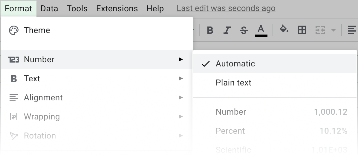
Note. This is required to avoid problems with formats on the next steps.
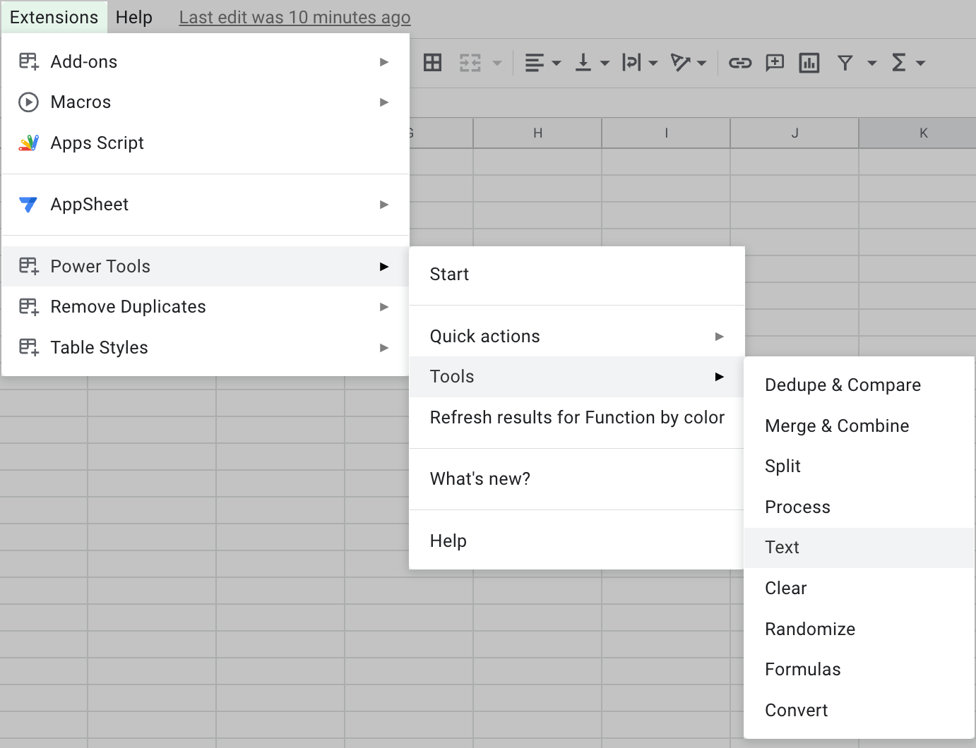
- Keep the values selected and run the Text tool from Extensions > Power Tools > Tools > Text:
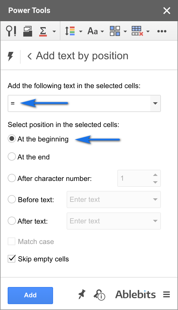
- Open Add text by position and add an equal sign (=) to add it at the beginning of each cell:
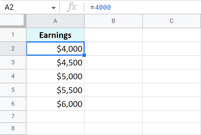
- Click Run to turn all your numbers to formulas:
- Proceed to the Formulas tool in Power Tools and select the option to modify all selected formulas.
You will see %formula% is already written there. You are to add those calculations you want to apply to all formulas at once.
Remember the formula to increase a number by percent?
=Amount*(1+%)Well, you already have those amounts in column A – this is your %formula% for the tool. Now you should only add the missing part to calculate the increase: *(1+10%). The whole entry looks like this:
%formula%*(1+10%)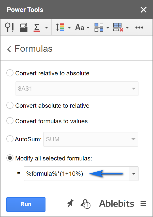
- Hit Run and all records will be raised by 10% at once:
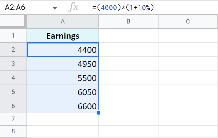
Tip. Feel free to apply any number format back to these formulas.
That's it! All these examples are easy-to-follow and are intended to remind those of you who've forgotten or show those who don't know the basic rules of calculating percentage in Google Sheets.
Spreadsheet with formula examples
Google Sheets percentage formulas - usage and examples (make yourself a copy)
 by
by 
196 comments
Hi,
I'm trying to do the percentage of a sum and I don't know which function to use for it. Here's my example:
Column A=10.62
Column B=5.50
Column C= 7.99 Percent of (A+B), 7.99% of (16.12) = 1.29 (rounded)
Does this make sense? I want C to add A and B together then find the percent of it.
Thanks!
Hi Anna,
Try this formula:
=ROUND((SUM(A1,B1)*C1)/100,2)
hello! mam,
i have a some values as a,
no. of quantity 12 and 150 rate and percent 30% = ans
means that
12*150/30%=ans
how to used formula.
Hello SHIVKUMAR,
I'm sorry, your question is not quite clear. If you specify what you're trying to calculate, I may be able to suggest a formula.
Hi Natalia,
14.75 13.25 12.30 11.40 10.75 10.10 9.50 8.95
15.25 13.70 12.75 11.80 11.10 10.45 9.85 9.25
15.75 14.20 13.20 12.25 11.55 10.85 10.20 9.60
- .80 - .30 -.30 -.10 -.10 -.10 -.10
This is a sample of the sheet I am doing. The first column is the main number each column after follows an =A1-(then amount on the bottom row) however, I need to have that formula less than 5% as well. I can't seem to get the additional 5% subtracted from that formula. How do I do that?
Hi Elizabeth,
Please try formulas from this part of the article. If they don't work, please show the exact formulas that you use, I'll try to help you.
After searching found this post with variety of cases and detailed explaination.. very useful.
I was searching variation of "Work out percent change from column to column" mentioned above but containing both positive and negative numbers in column. for example say [B ,C] columns cosist of
[-16,-13], [1,0.1],[-4,-8], [0.5,-1], [2,4],[-0.1, 0.5]. Could you please review and share your suggestion?
Hello Jagdish,
Thank you for your feedback!
Try dividing the subtraction to the absolute number using the ABS function:
=(C2-B2)/ABS(B2)
Or try a formula like this:
=(C8-B8)/AVERAGE(B8:C8)
Whichever one you choose, don't forget to apply the percent format.
How do I calculate 1 cell as a % of another cell? e.g. I should have 100 units but only have 80 units so the unit accuracy is 80%
Hello David,
If I understand your question correctly, the very basic percentage formula will help you out:
How to calculate percentage in Google Sheets
HI, super helpful, I need to see what 7% or any percentage eventually of a total volume goal. Each rep is assigned a goal, one reps is let's say 2000 for the month. how do a find a formula that will calculate each ones goal? hope that makes sense. thank you in advance
Hi David,
appreciate your feedback! If I get your task right, calculating percentage of a total should help you out.
If this doesn't help, please describe your task in more detail, I'll try to help.
Hello!
I am making a budget sheet, where I have a total income box and several different expense boxes, with the percent of total income for each. Is there a way to change the percent of one of the expense boxes and have one of the others automatically adjust its percent/dollar value so that total expenses don't exceed total income?
Thanks!
Hello William,
I'd advise you to look at the IF function. It looks like it should help you set up the correct percentage to display based on values from other cells.
if I want to calculate a % based on wins vs losses how would I do that?
I have a column of W's and L's for wins and losses and I want a formula that calculates the win % of all those cells
Hello Victor,
If I understand your task correctly, formulas to calculate the percentage of a total should help you. Otherwise, please describe your task in detail, I'll try to help.
I'm trying to add 20% to prices but want the people to just type in the amount and it to automatically add the 20% to it, how do I do this?
Example: the price is $10 but need to add 20% to make the amount show $12. Is there a formula I can put in the column to make this happen without adding another column to do the calculations in?
Hello Teri,
I'm afraid Google Sheets doesn't work like this. You can't enter the value and the formula for that value in the same cell. It's either one, so you will have to use an extra column with formulas referencing other cells.
I am trying to either create a pie chart or a percentage of the contents of a specific column. I have used conditional formatting and data validation to color the values in each row based on 5 possible answers. Now I need to know the percentage of each possible value.
For example, In one row I have several names, all different. In the next row, I have their choice: Red, blue, Green. How do I create a pie chart to show how many chose each color, or at least calculate a percentage?
Thank you!
Hello Jessie,
If you prefer the percentage, look for the example formulas here: Percentage of a total in a Google spreadsheet
If you'd like to have a Pie chart, the following tutorial should help: Pie Chart in a Google Spreadsheet
Hi
I'm trying to calculate the following, how can I do it.
I have a product's cost price, and selling price and would like to know what margin has been put on it, so for example if the cost price is $11.65 and the selling price is $18.95 what is the % profit made here.
Thanks very much
Abraham
Hi Abraham,
You will find the formulas to calculate percent change in this part of the article: Percentage increase and decrease formulas
I am fairly new with google sheets, but I was wondering if it would be possible to track sales over $12 and calculate a 12% tax on those sales? Basically we have a space that is rented to vendors, and any item priced $12 and above would be taxed a 12% fee. We have separate codes for each vender, and I am not entirely sure how we would input this into google sheets. If you could possibly help that would be wonderful! Thank you!
Hello Angel,
If I understand your task correctly, this part of the article will help you out: Increase and decrease numbers by percentage
Hi! I'm creating a spreadsheet to track our yearly sales in Real Estate.
Column B is Commission %, Column C is the Gross Sale Price and Column D is the actual dollar amount of the commission made.
How would I set something like that up to automatically calculate Column D? Thank you so much!
Hi Becca,
If I get your task right, use the formula from this section to do the math.
Hi there,
What would be the formula for having three columns of data (# of tickets sold today, # of tickets sold yesterday, % of total tickets available sold) and THEN a 4th column for percent increase or decrease from the 3rd column for that day?
So if our venue has a total of 580 seats and yesterday we were at 120 tickets sold (21%) and today we are at 150 tickets sold (25%), how can I show that ticket sales went up 4%?
I want to keep the column that shows today's percentage, but also shows how much ticket sales increased/decreased from yesterday.
Make sense? Thank you!
Hello!
If I understand your task correctly, the following formula should work for you:
=(C1-A1)/580
To understand how it works, please read through this part of the blog post: Percentage increase/decrease
Thank for the great resource!
I'm creating a simple budgeting spreadsheet for the wife and me. I can easily reference differences from one sheet to another (Example: (B4-('2021-11'!B4)) , where '2021-11' is the sheet for November 2021 and B4 is the cell I want a differential for).
Question: Is there a way to make this formula "portable" to auto-reference the sheet before it? I would like to not have to change the sheet name every month when updating.
Thank you in advance!
Thank you for the lovely words, Matt.
Yes, there's a way. You can incorporate INDIRECT, MONTH and TODAY functions to always subtract 1 from the today's month and reference the sheet for the previous month, like this:
=B4-INDIRECT("2021-"&(MONTH(TODAY())-1)&"!B4")
do you know how to sort by percentage? like 0.00% to 100.00%?
thanks
Hello Kenny,
Have you tried sorting A -> Z with the Google Sheets standard setting?
Is there a way I can format a percentage through a formula/function instead of doing it through the formatting toolbar?
I have this formula and want to make sure the % output is formatted as having two decimal places.
ex. 1.12% instead of just outputting 1%.
I have the formatting set to "Automatic" as the same cell is used to output a $ amount depending on the contents of another cell. When the contents of that cell has a certain criterion, a % will show up, which it is doing so correctly, but it's showing up as rounded and i want it to show two decimal places.
to_percent(A2/A1)
Thanks
Jenny
Hello Jenny,
Try the Google Sheets ROUND function.
I got this from investopedia.com which says you have to switch numbers in the formula if the price decreases or increases:
Understanding Percentage Change
Percentage change can be applied to any quantity that you measure over time. Let's say you are tracking the quoted price of a security. If the price increased, use the formula [(New Price - Old Price)/Old Price] and then multiply that number by 100. If the price decreased, use the formula [(Old Price - New Price)/Old Price] and multiply that number by 100.
this is totally confusing....
Hello les,
I explained the percentage change in this part of the blog post, please have a look.
Hello!
Amazing article that's been super helpful!
I'm trying to make a tracker on sheets that follow progress of workouts for a group.
Having to do pull ups, push ups sit ups, etc.. then trying to equal that into a 100%
Example:
5 of 15 push ups, 10 of 10 sit ups, and 15 of 15 pull ups = 75%(?) Not great at math...
Thanks for taking a look at my request for help!
Thank you for your feedback, Jon!
Since I don't know how you arrange your data, I can only hint on the steps to calculate. You'll need:
Then you'll be able to find the percentage as described here.
My Rat Turd sized brain still doesn't understand plz help
Hello Makayla,
You can describe your task in detail and I'll see if I can suggest you anything.
If I wanted to create a budget spreadsheet, and have Google Sheets calculate the percentages of my check to put away, which one would I use above? So for example, if I want to put in my income as $2000 and have it calculate 70% savings, 20% bills and 10% entertainment for me. Thanks!
Hello Lisa,
I believe Amount and total by percentage will help you out.
Hi,
I am trying to highlight the cells in column L that DO NOT fall within a certain percentage : between -30% of J2 and +30% of J2
basically, if value in L2 is NOT within a 30% range (under or over) the value in J2, Then turn the row in RED
I tried this =and(L2>=0.9*J2,L2>=1.1*J2) in Conditional formatting, but it doesn't seem to be working
Any help will be greatly appreciated.
Hi Najon,
Try this rule instead:
=AND(L2>=0.7*J2,L2<=1.3*J2)
can someone help me with this formula ?
=ARRAY_CONSTRAIN(ARRAYFORMULA(IF($E3:E970*F$1>0, IF($D3:$D970<=EDATE($C3:C970,12),$E3:E970*F$1,""),"")), 968, 1)
Hi,
Please describe your task in detail and specify what error your formula returns.
i figured it out, sort of lol
=to_percent((b105:b135-D105:D135)/D105:D135)
just had to put it in every cell instead of (g) instead of doing a range
Hello Mike,
To check your cells for conditions first (if X sold N last week and N this week), you need to incorporate the IF function. The % increase will be used as a second argument and will happen only if the conditions are true.
Also, you can calculate this for all rows at once by enfolding the formula in ARRAYFORMULA.
i am trying to figure out a way to make a contest for my employess by amount of sales weekly percentage increase (or decrease)
i.e. if bob (B105) sold $19876 (D105) last week, and sold 21000 (E105) this week, his % increase would be =X
is there a way to do this for a whole range... or just line by line?
as if there were 33 employees, bob being first on 105, and debra being last on 138
i hope this makes sense?!?!
thanks in advance!
i figured it out, sort of lol
=to_percent((b105:b135-D105:D135)/D105:D135)
just had to put it in every cell instead of (g) instead of doing a range
Hello! Thank you for this wonderful resource. I have a chart I need to frequently generate, and am stumped with how to auto populate a certain column. Column A is a date range (fine), Column B is the days within Column A as just numbered 1-->whatever (fine), Column C is data I enter with daily measurements (fine) but the starting number is what controls what I need in Column D and subsequent columns with varying percentage reduction. What I need to figure out is how to take a starting number (call it SN, which begins all the columns I need to auto populate) then take a percentage of that, divide that amount by the number of days in the date range, and subtract sequentially down that column. Example: 3956 SN, take 18% of that (712.08), then divide that amount by 12 days (59.34), each day subtracting another 59.34 while generating a line. The purpose of this is to have a quick, and visual, representation of how daily measurements compare to several ideal percentage reductions, allowing me to adjust the environmental parameters in the project. I am embarrassed to admit I have been doing the calculations and manually entering the results in each cell! This is not good. It's been decades since I've been regularly doing work with spreadsheets and this old brain needs help. Thank you.
Nevermind . . . I figured it out! Thanks again for having this site.
Thank you for the lovely feedback! Glad to know you've found the solution :)
I am trying to convert my grades to percents using this form. For example, the sheets generate the score as a number out of the total like: 4/20. How do I get it to create the percentage for each score?
Hello Beckie,
Assuming your total is generated in A2, a formula like this should help:
=INDEX(SPLIT(A2,"/"),1,1)/INDEX(SPLIT(A2,"/"),1,2)
Don't forget to apply the Percentage format to your cell with the formula.
Your calculation to find the original price for a 40% discounted scooter is incorrect. Your calculation is 1500/.4 and it should be 1500/.6.
Oh my! Thank you, Curtiss, I've corrected the info :)
=SOM(B1-A1)/B1 x100
not working
4,1 - 3,5 = 0,6 : 3,5 = 0,171x 100 = 17%
Or :
3,5 -4,1 = -0,6 : 4,1= -0,146x100=-14,6%
Hi Ruud,
Your formula is written incorrectly:
Hence, here's how a correct formula should look:
=(B1-A1)/B1*100
I don't understand
Hello Amir,
You're welcome to describe your task here, I'll see if there's an easy solution and suggest where to look.
Hello,
I am looking for A1 to show a percent value of B1 after it surpasses 5000. I also only want the percent value to be of all values added after 5000.
A1=25%B1>5000
As in:
If B1=6000 then A1=250
Is this possible? I'm a bit new to this level of function use and am having trouble sorting through what I am able to do. So far I have had to create a separate key of cells that show the percentage I want to apply to B1 per other cell I want to show said value. For reference this is meant for a royalties accounting spread sheet that has several individuals receiving a different percent of profit per music release so there are a lot of variables and it makes it really messy to try and have a separate key for percentages and alternate cell values. Not sure if this all makes sense? Thank you for this awesome resource!!
Hello Cameron,
If I understand your task correctly, this formula (using the IF function) may help:
=IF(B1>5000,(B1-5000)*0.25,"")
A very good explanation of formulas. This will help to a great extent those who are working on excel. Truly fantastic article. Thanks for sharing this. Kudos!!!
hey there!
I need help regarding a problem I'm having with sheets. I have a table that has Months (from Jan to Dec) in the X axis and the name of the asset in the Y axis. I want to add the new value of the asset under each month and I want sheets to indicate (in a column at the end of the table) the growth rate it has had from the very first month. I would like if I didn't have to keep changing manually the formula of said column. Is there someway it can do so automatically?
I would really appreciate your replies,
Cheers!
Hey Deidara,
If I understand you correctly, you can use ArrayFormula in the last column to calculate all rows, existing and future ones, automatically. If this is not exactly what you need, please describe the task in more detail.
You can also share an editable copy of your spreadsheet with us (support@apps4gs.com) with 2 sheets: a copy of your source data and the result you expect to get. I kindly ask you to shorten the tables to 10-20 rows.
Note. We keep that Google account for file sharing only, please do not email there. Once you share the file, just confirm by replying here.
مرحبا
H3=مبلغ
I3=5% نسبة
=H3*I3
يعطني خطاء
لماذا
Hello Abdel,
Can you please provide the exact formula you have in H3 and the result it returns?
Hi there,
Thank you so much for creating useful content and helping me thereby solving my google spreadsheet question. Thanks again!
Hello,
I have the same problem as the person below did on 11/19/19. I will enclose my formulas.
These formulas gave me 98% COUNTIF(E5:E107,"No")/COUNTA(E5:E107,"no") =COUNTIF(E5:E107,"Yes")/COUNTA(E5:E107,"Yes")
This formula gave me a 99% =COUNTIF(H5:H107,"No")/COUNTA(H5:H107,"No")
=COUNTIF(H5:H107,"Yes")/COUNTA(H5:H107,"Yes")
Hi,
I'm trying to keep track of attendance using a google sheet with checkboxes. Here is the formula for what I have: =COUNTIF(C6:X6,"TRUE")/COUNTA(C6:X6,"FALSE")
My issue is, if all of the boxes are checked, the percent should be 100% but it's only 95.65%.
Hello Martha,
COUNTA counts all non-empty cells within the range no matter their contents. The values you're using as the second argument ("FALSE" or "no") don't tell what to count. The second argument is also a range to count, so these records are actually counted as "1" mixing the numbers up.
So please change all your COUNTA to COUNTIF and everything should work correctly then.
Thanks for providing a great resource. I have a table of columns and rows with sales figures that go up and down. Using formulas, the table displays monthly changes in sales as percentages. I have them color-coded so sales increases display in green and decreases display in red. The decreases show a minus character (-) automatically. Is there a way to automatically display an addition character (+) for a percentage increase? Thanks!
Thank you for your feedback, Trevor.
You will need to select your cells with the percentage increase and create a custom number format like this: "+"0%
Thank you. Is there any way to make the "+" automatically appear only in cases where a percentage exceeds 0.00%?
Trevor,
Try this custom number format instead:
[<0]"-"0.00%;[>0]"+"0.00%;0.00%
Hi -
I have a number of identical laid-out sheets and have the same metric in each = open rate as a percent.
In my summary sheet, I want to calculate the average percent across the sheets.
Hi Derek,
If I understand your task correctly, it is the AVERAGE function that will help you.
You will need to refer to cells from each sheet though to collect and calculate everything correctly.
Hello!
I'm looking to calculate a shopping spreadsheet and would like to calculate discounts & taxes. What formula can I use to calculate total + 15% tax for example?
Hello Elyse,
Assuming your total is in column A and tax is in column B, you can try this formula:
=A2+(A2*B2)
The multiplication in brackets is used to find the amount of the tax, then it is added to the total in column A giving you a sum you will need to pay.
Such a great article. I'm trying to increase a number in cell by a percentage and it doesn't seem to be working. i used the fomula you stated but it adds the percentage as 100% and not 10%. Any ideas as to why that is?
I appreciate it,
Adkins
Hello Adkins,
Can you please provide the exact formula you use in your sheet that returns the incorrect result?
need to calculate percentage markup
row of cells: cost retail %markup
need to multiply cost x100 then divide by retail? just can't figure out order
Hello Kirsting,
Try to subtract the original cost from the retail, then divide it by the cost, and then multiply by 100.
Please refer to this web-page for more details:
https://corporatefinanceinstitute.com/resources/knowledge/accounting/markup/
Hi! thank you for this tutorial!
You may be able to help me, I am doing a spreadsheet where I track my business profits on a daily basis.
I already get my daily % growth, but I would like to do a TOTAL percentage, from my 1st day to today.
The trick is that I want it to fill itself, and in only 1 cell. I want the result of this growth to always appear in the 'k5' cell, for example, and for it to always take the last input and the very 1st one without me having to change the formula every day.
If you can help, I'll take it!
Thank you very much.
Hi Kuro,
thank you for the feedback!
I'm afraid I'll need more details on your data to help you out. Can you please describe where it's located in the spreadsheet in detail (Sheet? Column? The number of rows?) and give an example of how it looks?
What formula do you use and what do you update in it constantly?
My family and I have a weekly running nfl pool. Each week column input and results of course change. I use check boxes to say who wins and who loses and the sumif function at the end of the column to give me the needed results. I decided to test the workings of the sheet and everything works fine except for one thing. When I attempt to divide cells d22(total wins) with e22(total losses) To get the percentage needed I have used the formula =(D22+E22)/D22 which does not work. What am I doing wrong?
Joseph,
Could you please specify what are you trying to get? The percent of losses or wins from the complete total? Or something else?
If it's possible, please also share your sample data with us (support@4-bits.com) and reply to my comment when we can take a look. Thank you.
I disabled my ad blocker, so much good content thanks for sharing.
Hi,
I'm trying to keep track of attendance using a google sheet with checkboxes. Here is the formula for what I have: =COUNTIF(C6:X6,"TRUE")/COUNTA(C6:X6,"FALSE")
My issue is, if all of the boxes are checked, the percent should be 100% but it's only 95.65%.
Any ideas?
Hi Lisa,
Would you mind sharing your sample data with us (support@4-bits.com) so we could have a look?
Note. That email address' Inbox is unmonitored. Once you share the file, please confirm by replying here. Thank you.
Hi,
How to do calculate =a2*b2 for multiple cells ex:a2-a5*b2-b5 etc...
Hi Matt,
If I understand you correctly, this formula should do the trick:
=ARRAYFORMULA(A2:A5*C2:C5)
Why does google sheets add 2 zeros to my values when I try to apply the "percent" format?? I just want the % to appear next to the number already in the cell.
Hello Diana,
That's simply the way Google Sheets works.
In your turn, you can adjust the number of zeros using the corresponding options from the Sheets toolbar. Look for two buttons with zeros right under the Format option: Decrease decimal places and Increase decimal places. The tip from this point of the article shows them.
or do a vidio please
Hello Tyler,
Could you please specify what points of the article remain unclear?
At the moment I don't believe the video would feature something other than the same formulas.
If you could describe the task you're dealing with, I would gain a better understanding of what to improve.
Thank you.
Hey so I run a business and I pay my drivers 30% of the income. Lets say a driver makes on a week $4560 I need to pay 30% of that to him. Is there a formula that can help me find the value of that 30%? Thank you.
Hi Daymaris,
You'll find the required formula in the following part of the blog post above: Amount and total by percentage in Google spreadsheets
Can you do a dumbeddown version of this please because my penut sized brain dosent understand
Great stuff!
Thank you! :)