In this tutorial, you will learn how to create a number sequence in Excel with formulas. Additionally, we'll show you how to auto generate a series of Roman numbers and random integers - all by using a new dynamic array SEQUENCE function.
The times when you had to put numbers in sequence in Excel manually are long gone. In modern Excel, you can make a simple number series in a flash with the Auto Fill feature. If you have a more specific task in mind, then use the SEQUENCE function, which is specially designed for this purpose.
Excel SEQUENCE function
The SEQUENCE function in Excel is used to generate an array of sequential numbers such as 1, 2, 3, etc.
It is a new dynamic array function introduced in Microsoft Excel 365. The result is a dynamic array that spills into the specified number of rows and columns automatically.
The function has the following syntax:
Where:
Rows (optional) - the number of rows to fill.
Columns (optional) - the number of columns to fill. If omitted, defaults to 1 column.
Start (optional) - the starting number in the sequence. If omitted, defaults to 1.
Step (optional) - the increment for each subsequent value in the sequence. It can be positive or negative.
- If positive, subsequent values increase, creating an ascending sequence.
- If negative, subsequent values decrease, producing a descending sequence.
- If omitted, the step defaults to 1.
The SEQUENCE function is only supported in Excel for Microsoft 365, Excel 2021, and Excel for the web.
Basic formula to create a number sequence in Excel
If you are looking to populate a column of rows with sequential numbers starting at 1, you can use the Excel SEQUENCE function in its simplest form:
To put numbers in a column:
To place numbers in a row:
Where n is the number of elements in the sequence.
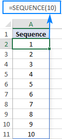
For example, to populate a column with 10 incremental numbers, type the below formula in the first cell (A2 in our case) and press the Enter key:
=SEQUENCE(10)
The results will spill in the other rows automatically.
To make a horizontal sequence, set the rows argument to 1 (or omit it) and define the number of columns, 8 in our case:
=SEQUENCE(1,8)

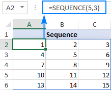
If you'd like to fill a range of cells with sequential numbers, then define both the rows and columns arguments. For instance, to populate 5 rows and 3 columns, you'd use this formula:
=SEQUENCE(5,3)
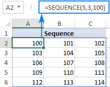
To start with a specific number, say 100, supply that number in the 3rd argument:
=SEQUENCE(5,3,100)
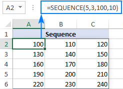
To generate a list of numbers with a specific increment step, define the step in the 4th argument, 10 in our case:
=SEQUENCE(5,3,100,10)
Translated into plain English, our complete formula reads as follows:

SEQUENCE function - things to remember
To efficiently do a sequence of numbers in Excel, please remember these 4 simple facts:
- The SEQUENCE function is only available with Microsoft 365 subscriptions and Excel 2021. In Excel 2019, Excel 2016 and earlier versions, it does not work since those versions do not support dynamic arrays.
- If the array of sequential numbers is the final result, Excel outputs all the numbers automatically in a so-called spill range. So, be sure you have enough empty cells down and to the right of the cell where you enter the formula, otherwise a #SPILL error will occur.
- The resulting array can be one-dimensional or two-dimensional, depending on how you configure the rows and columns arguments.
- Any optional argument that is not set defaults to 1.
How to create a number sequence in Excel - formula examples
Though the basic SEQUENCE formula does not look very exciting, when combined with other functions, it takes on a whole new level of usefulness.
Make a decreasing (descending) sequence in Excel
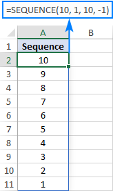
To generate a descending sequential series, such that each subsequent value is less than the preceding one, supply a negative number for the step argument.
For example, to create a list of numbers starting at 10 and decreasing by 1, use this formula:
=SEQUENCE(10, 1, 10, -1)
Force a two-dimensional sequence to move vertically top to bottom
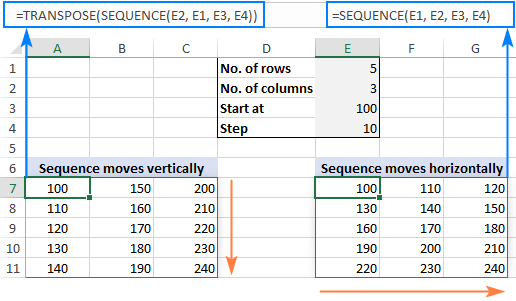
When populating a range of cells with sequential numbers, by default, the series always goes horizontally across the first row and then down to the next row, just like reading a book from left to right. To get it to propagate vertically, i.e. top to bottom across the first column and then right to the next column, nest SEQUENCE in the TRANSPOSE function. Please note that TRANSPOSE swaps rows and columns, so you should specify them in the reverse order:
For example, to fill 5 rows and 3 columns with sequential numbers starting at 100 and incremented by 10, the formula takes this form:
=TRANSPOSE(SEQUENCE(3, 5, 100, 10))
To better understand the approach, please have a look at the screenshot below. Here, we input all the parameters in separate cells (E1:E4) and create 2 sequences with the below formulas. Please pay attention rows and columns are supplied in different order!
Sequence that moves vertically top to bottom (row-wise):
=TRANSPOSE(SEQUENCE(E2, E1, E3, E4))
Regular sequence that moves horizontally left to right (column-wise):
=SEQUENCE(E1, E2, E3, E4)
Create a sequence of Roman numbers
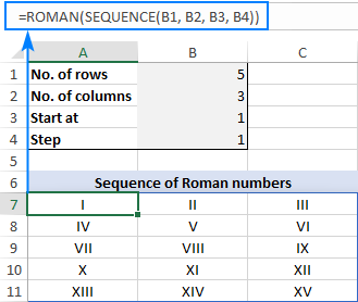
Need a Roman number sequence for some task, or just for fun? That's easy! Build a regular SEQUENCE formula and warp it in the ROMAN function. For example:
=ROMAN(SEQUENCE(B1, B2, B3, B4))
Where B1 is the number of rows, B2 is the number of columns, B3 is the start number and B4 is the step.
Generate an increasing or decreasing sequence of random numbers
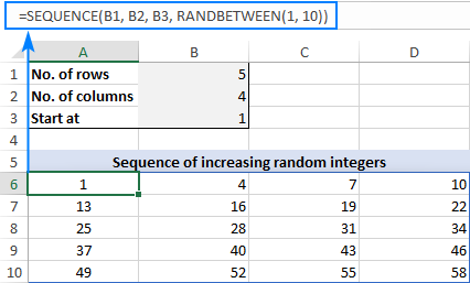
As you probably know, in new Excel there is a special function for generating random numbers, RANDARRAY, which we discussed a few articles ago. This function can do a lot of useful things, but in our case it cannot help. To generate either an ascending or descending series of random whole numbers, we'll be needing the good old RANDBETWEEN function for the step argument of SEQUENCE.
For example, to create a series of increasing random numbers that spills in as many rows and columns as specified in B1 and B2, respectively, and start at the integer in B3, the formula goes as follows:
=SEQUENCE(B1, B2, B3, RANDBETWEEN(1, 10))
Depending on whether you want a smaller or bigger step, supply a lower or higher number for the second argument of RANDBETWEEN.
To make a sequence of decreasing random numbers, the step should be negative, so you put the minus sign before the RANDBETWEEN function:
=SEQUENCE(B1, B2, B3, -RANDBETWEEN(1, 10))
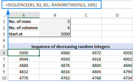
Note. Because the Excel RANDBETWEEN function is volatile, it will generate new random values with every change in your worksheet. As the result, your sequence of random numbers will be continuously changing. To prevent this from happening, you can use Excel's Paste Special > Values feature to replace formulas with values.
Excel SEQUENCE function missing
Like any other dynamic array function, SEQUENCE is only available in Excel for Microsoft 365 and Excel 2021 that support dynamic arrays. You won't find it in pre-dynamic Excel 2019, Excel 2016, and lower.
That's how to create sequence in Excel with formulas. I hope the examples were both useful and fun. Anyway, thank you for reading and hope to see you on our blog next week!
Practice workbook for download
Excel SEQUENCE formula examples (.xlsx file)
 by
by
399 comments
Bonsoir,
comment créer cette séquence :
LS-001/24
LS-002/24
LS-003/24
...
....
...
LS-500/24
Hi! Write numbers with leading zeros using TEXT function. Combine strings of text by using the & operator or any other method. Read more: Excel CONCATENATE function to combine strings, cells, columns.
The formula might look like this:
="LS-"&TEXT(SEQUENCE(10,1,1,1),"000")&"/24"
Hi! I'd like to create rows that has a pattern like this...
00001-00010
00011-00020
00021-00030
00031-00040
up to 15990-16000
I was wondering which formula to use. Thnak you!
Hi! Use the TEXT function to write numbers with leading zeros. Combine text strings using the & operator or other method.
For example:
=TEXT(SEQUENCE(10,1,1,10),"00000") & "-" & TEXT(SEQUENCE(10,1,10,10),"00000")
Thank you for your help!
Need sequence like below: could you please help me.
1 01-02-2024 S1
2 01-02-2024 S2
3 01-02-2024 S3
4 02-02-2024 S1
5 02-02-2024 S2
6 02-02-2024 S3
7 03-02-2024 S1
8 03-02-2024 S2
9 03-02-2024 S3
Hi! As I wrote earlier in the comments, you can create a sequence of repeating numbers or dates using the CEILING + SEQUENCE function.
To create a repeating sequence of numbers from 1 to 3, use the MOD and TRUNC functions.
Try these formulas:
=DATE(2024,2,1)+CEILING(SEQUENCE(100,1,1,1)/3,1)-1
="S"&TRUNC(MOD((SEQUENCE(100,1,1,1)-1)/1,3)+1)
I hope this will help.
is there any logic to create a conditional sequence as shown below?
Sl.No. Ref
1.1 aa
1.2 aa
1.3 aa
2.1 ab
2.2 ab
3.1 abc
3.2 abc
3.3 abc
3.4 abc
Hi! If there is some logical sequence in your data, describe it. Then I can understand what you want to do. Also note that you can create a sequence of digits using the SEQUENCE function.
mentioned is the sample of logical sequence.
Sl.No. Band Product
1.1 Dell Laptop
1.2 Dell Monitor
1.3 Dell NUC
2.1 Lenovo Laptop
2.2 Lenovo Tablet
3.1 Apple i-Phone
3.2 Apple i-Pad
3.3 Apple i-Mac
3.4 Apple i-Watch
As I said, I don't see any logical sequence in your data. Describe it if you can.
I'm using the SEQUENCE function to make a dynamic calendar that is auto populated by the year input. My formula is =SEQUENCE(1,7,DATE(C2,1,1)-WEEKDAY(DATE(C2,1,1))+1,1). It works out great however I would like the sequence to skip every other row so I have room to add items to my calendar. How can I do this?
Hi! Based on your description, it is hard to completely understand your task. To understand what you want to do, tell me what is written in cell C2 and give an example of the desired result.
i believe he is looking for
a1 15 jan
a2
a3 22 Jan
a4
a5 29 Jan
there is an empty line after each auto filled seq line, so we can fill in information/ make notes like how we have on paper calendar
Hi! Specify the starting date using the DATE function. Using the formula CEILING(SEQUENCE(50,1,0,1)/2,1)*7, add the numbers 0 7 7 14 14 14 21 21 21 and so on consecutively to this date. This formula will generate a sequence of 50 numbers, starting from 0. The CEILING function rounds each number in the sequence up to the nearest integer that is divisible by 1. This effectively rounds up each number to the nearest whole number. The result is then multiplied by 7.
The formula (IF(MOD(SEQUENCE(50),2)=0,0,1)) will generate a sequence of numbers 0 1 0 1 0 1 0 1 0 1 0 1 and so on in the cells. The SEQUENCE function generates a sequence of numbers from 1 to 50, and the MOD function checks if each number in the sequence is even or odd. If the number is even, the formula returns 0, and if the number is odd, the formula returns 1.
=(DATE(2024,1,15) + CEILING(SEQUENCE(50,1,0,1)/2,1)*7) * (IF(MOD(SEQUENCE(50),2)=0,0,1))
To show dates in the format you want and not show zeros, set a custom date format in the cells: dd mmm;;
Thank you for your help. It is greatly appreciated!
Hi there, I'm attempting to generate a sequence where the number of rows is dependent on Column A, with only one Column, starting with 0, and increment step is 1.
Column B has an identifier that repeats for every like row. For example, in the case of multiple Contact records under one Company, the Company in this case would repeat in Column B, where each Contact Record would be unique in Column A.
The sequence I want to apply would start over from 0 once Column B no longer repeats. The output would be in Column C. Please see the example table below of my desired outcome.
Contact Company Sequence ID
5991 416 0
4565 416 1
1790 416 2
1761 416 3
1023 416 4
6924 417 0
4770 417 1
4640 417 2
1309 418 0
7773 418 1
2682 419 0
7898 419 1
8310 419 2
1209 419 3
1314 419 4
How do I achieve the output in Column C?
Hi! I think you can count the number of duplicates in column B using the COUNTIF function and subtract 1 from the result. Read more: How to count duplicates in Excel.
=COUNTIF($B$1:B1,B1)-1
I hope my advice will help you solve your task.
hello sir
i want to make sequence of digits which are with alphabets like ( PLR-101-1) how can i do this please help me out. and if the article is change like ( Thu-508--Set) then how can i make the center digit sequence ?
Hello! If you read the comments above, you will see many such examples. Combine text strings with a SEQUENCE formula using the concatenation operator (&). For example:
="Thu-"&SEQUENCE(10,1,508,1)&"--Set"
Hi.
I want to create a dynamic numbering for some kind of Database for Samples.
I got an Input Table where i write the basic informations in. Then i write the total Number of Objects.
Object1 4
Object2 3
Now i want to create a Dynamich numbering in a list where i have following collumns
Intern ID Position Date Sample Number Samples Name
after the 4th Sample for Object 1 it should start with the First Sample of Object 2
Hi! Please clarify your specific problem or provide additional information to understand what you need.
I have 3 columns of numbers data . The device count changes, The AMP and channel is always the same. I was trying to see if a =sequence function would work but not figuring it out if so.
AMP Channel Device Count
1 1 20
1 2 1
1 3 10
1 4 5
1 5 2
1 6 3
1 7 7
1 8 9
2 1
2 2
2 3
2 4
I need to create a column that looks like
1-1-1
1-1-2
to
1-1-20
1-2-1
1-3-1
to
1-3-10
ect
Any help would be great thanks.
Hi! There are many such examples in the comments above. Read it. Combine a sequence of values with text using the concatenation operator &. For example.
="1-1-"&SEQUENCE(20,1,1,1)
Thanks for that help, Is there a way to get it then to continue and the second number change after 20 entries, to 1-2-1? I worded it wrong maybe above.
Hi! I advised you to read the comments above. Too bad you didn't. To repeat each number of the sequence 20 times, use the formula:
=CEILING(SEQUENCE(80,1,1,1)/20,1)
To repeat the sequence several times, use the formula
TRUNC(MOD((SEQUENCE(80,1,1,1)-1)/1,20)+1)
Concatenate into a text string using & operator:
="1-"&CEILING(SEQUENCE(80,1,1,1)/20,1)&"-"&TRUNC(MOD((SEQUENCE(80,1,1,1)-1)/1,20)+1)
How to generate consecutive numbers starting from 43 to 60 and each number should repeat 5 times.
For example
column A
43
43
43
43
43
44
44
44
44
44
45
45
45
45
45
and
upto 60 ?
Hi! You can find many such formulas in the comments above:
=CEILING(SEQUENCE(50,1,1,1)/5,1)+42
Hello,
I want to create a reference number formula in an excel cell in a payment voucher such that when I save one payment voucher and I close and open the payment voucher again, It will increment itself.
Thank you.
Hi! Unfortunately, without seeing your data, it is difficult to give you any advice. Please provide me with an example of the source data and the expected result.
Hello
I'm attempting to link two different spreadsheets, one being a view/ work-log, the other is an entry-log. The work-logs only purpose is to calculate the remaining dollar amount and percentages. The entry-log is an ongoing form that totals around 50 individual sheets, which means every new entry will differ. The entry-log will only use 7-12 cells that reflect on the work-log in sequential order. The problem I'm having is how to add a traspose fx that will work in sequence with the two forms to prevent me from having to link them manually for each sheet?
Is it possible to add a sequence with this formula below without removing the transpose fx?
=TRANSPOSE('[Weatherization - Joshen RFP.xlsx]JOSHEN '!$C$14:$C$17)
Hello! It is very difficult to understand a formula that contains unique references to your data, which I don't have. Unfortunately, I can't understand what you want to do.
hi,
I have three columns : employee, salary (yearly), startdate. I want to generate a provisional monthly cashflow table for the next 3 years with three columns : employee, payment (monthly), paymentdate.
I know how to this using SEQUENCE for one employee but is there a way to generate it at once for several employees ? In other words, this would be the same as generating sequence lines one below the previous.
Thanks
Hi! You can create only one sequence using the SEQUENCE formula.
Hi,
I have CSV data that has been loaded into Excel using the common method under the Data / From Text menu, into a separate worksheet labelled "Raw Data". I want to paste this data into another worksheet from a start position identified as "1". The simple formula used to achieve the "1" starting position is =IF(CE$4=BJ695,1,""), where CE$4 is time in DD/MM/YYYY hh:mm:ss format and BJ695 is one of a series of cells with the same time format. The time is in sequential order in column BJ. The formula identified places a "1" as the starting position in column "CE". In the adjacent column "CD" the data from the worksheet "Raw Data" should start. I have tried Index Match formulae to no avail and am losing my mind over this. Is there a simple way of completing this task without introducing many more helping columns, as the worksheet is already large? I would greatly appreciate any help provided.
Many thanks... Damian.
Hi! Dates that you load to Excel from a CSV file, are usually not written as dates, but as text. Check this and use these guidelines: How to convert text to date in Excel. I hope it’ll be helpful.
Can I use the sequence function if I want to repeat number 12 times then incrementing 1 until I reached 24 it goes back to number 1? Thanks
I don't think this can be done with a sequence function. Write down 24 numbers and copy them as many times as necessary.
Hi , I want to apply a function on a generated sequence. Say there are 5 numbers {1,2,3,4,5} , I want harmonic sum of each the numbers in the sequence and then I want cumulative sum of the results. How will it be possible ?
Hi! Please clarify your specific problem or provide additional information to understand what you need. Maybe this article will be helpful: How to do a running total in Excel (Cumulative Sum formula).
Hi ,
Seek your guidance how shall i proceed built the sequence formula for below scenario in excel template
1.scenario 1
13/9/ABC/01
13/9/ABC/02
13/9/ABC/03
13/9/ABCa/04
13/9/ABC/05
13/9 > referring to DD/MM base on today/weekday case ID receive
ABC - defaulted
01 - refer to sequence number for each entry of the row
2. Scenario 2 sequence format
202309120001
202309120002
202309120003
202309120004
"20230912" - referring to current request date receive for the data entry
"0001", 002,003 - referring to sequence number of request received for the day
if the subsequent date no request, then will no case ID generate
Assume case receive on 20230915, then the case ID number will be 2020309150001.....follow by 202309150002...etc
Thank you.
Hi! Use the TEXT function to write dates and numbers in the desired format.
=TEXT(A1,"mm.dd")&"."&"ABC/"&TEXT(SEQUENCE(10,1,1,1),"00")
thank you so much on your useful tips.
The serial number working perfectly for Date 9 Oct 2023. However, when is new date eg: 10 Oct 2023, 11 Oct 2023, the sequence number is not reset start with "0001". Expected format shall be 10/10 ABC/0001, 10/10 ABC/0002.....etc if there is new date 11 Oct 2023 then shall be 11/11 ABC/0001, 11/11 ABC/0002....etc. Can this be done with formula?
9-Oct-23 09/10 ABC/0001
9-Oct-23 09/10 ABC/0002
9-Oct-23 09/10 ABC/0003
9-Oct-23 09/10 ABC/0004
9-Oct-23 09/10 ABC/0005
10-Oct-23 10/10 ABC/0006
10-Oct-23 10/10 ABC/0007
12-Oct-23 12/10 ABC/0008
13-Oct-23 13/10 ABC/0009
Thank you.
Hi! Based on your second description, it is not about creating a sequence. You need to create code for each new record. You can use the COUNTIF formula for dates to determine the ordinal number of the record within each day. Unfortunately, without seeing your data, it is impossible to offer you a formula.
I need to create a sequence that consists of two columns, the first being Serial No., which contains sequence 1 to 100,000. Columns. 2 is having a code that will have a format based on the serial number value from column 1, i.e., 1 to 1000, code value will be 1, column 1001-2000 column 2 value is 2, which means after each 1000 the code value will change. Can you please help find a simple way to do that?
Hi! You can find the formula for the first column in the article above. For the second column, you can use the rounding to thousands formula:
=ROUNDUP(A1/1000,0)
Or you can use the sequence formula, as has been described many times in the comments to this article:
=CEILING(SEQUENCE(100000,1,1,1)/1000,1)
How wil autogenerate responses for 200 respondents, already have for 55 responses in excel
i have a set of responses from 55 respondents, but i need like 200 ,how will i autogenerate the remaining responses .
Is it possible
300/7/2023
301/7/2023
302/7/2023
303/7/2023
Hi! Create a sequence as described in the article above and add a text string using the & operator.
=SEQUENCE(10,1,300,1)&"/7/2023"
Hello, I have these names in A1:A8 and need to enumerate them on C1:C8, excluding the ones that say treasury. The sequence also depends on the year selected in B1:B8
A B
1 Other property 2023
2 Passenger vehicle 2023
3 Non-passenger vehicle 2023
4 Treasury 2023
5 Other Property 2023
6 Non-passenger vehicle 2024
7 Treasury 2024
8 Non-passenger vehicle 2024
Expected sequence in C
1 01
2 02
3 03
4
5 04
6 01
7
8 02
Hi! The expected sequence you described is not very clear to me. Also note that you will be able to use the year if it is written in a separate column as a number.
Hello, Unfortunately I'm stuck with Excel 2016 and unable to use the SEQUENCE function. Do you have any recommendations for a formula that will create a list of numbers between two values, separated by a certain number? For example, all numbers between 8000 and 10000 seperated by 5. I'll need to do this many times and a formula would be extremely helpful!
Hello! To create a sequence of numbers, you can use the ROW function. The ROW function returns the row number. For example:
=80000+(ROW(A1)-1)*5
Copy this formula down the column.
Hi Alexander,
How to sequence the following please:
K0151/right
K0151/left
K0152/right
K0152/left
K0153/right
K0153/left
I am not good at it. Thank you for your help!
Hi! The formula below will do the trick for you:
="K" & TEXT(CEILING(SEQUENCE(45,1,1,1)/2,1)+150,"0000") & CHOOSE(MOD(SEQUENCE(45,1,1,1),2)+1,"/left","/right")
Hi, How do I sequence with sequence no depends on value on multiple cells/columns, for example:
Col-A Col-B Col-C Col-D (which is the sequence, which value starts can be random value), Thanks a lot!
111 RP C 05
111 RP C 06
AAA DW R 25
111 RP C 07
AAA DW S 55
AAA DW S 56
111 RP C 08
Hi! With Excel formulas, you can only make a sequence of numbers. You have text. Also, there is no pattern in your data that can be written as a formula.
I have a question, please help if you can.
I need a particular pattern in which every number -start from number 1- exist in every successive 5 cells in one column like from A1 to A5 filled with number 1
From A6 to A10 filled with number 2 and so on.
How can I do this?
Thanks in advance
Hi! If I understand your task correctly, try the following formula:
=CEILING(SEQUENCE(50,1,1,1)/5,1)
Hi,
How to convert range (column A1 to B2) into array in single cell for word office 365?
Example:
A1=4
B1=8
Convert array in single cell like this
Result: {4;5;6;7;8}
note:
Previous version word use below formula but not work on office 365.
{ =ROW(INDIRECT(A1&":"&B1)) }
Hi! Brackets are not needed in this formula: =ROW(INDIRECT(A1&":"&B1))
In previous versions of Excel, this formula was written as an array formula. In Excel365 you don't need to do this.
Hello,
I'm after a sequence for creating quote numbers, It would take the Year (2023) Month (04) - then a numerical sequence from 1 down till X.
From the date the quote was provided.
Unless the next month starts, then it would be 2023-05-1, etc
Say Cell Values of 2023-04-1, 2023-04-2, 2023-04-3, 2023-05-1, 2023-05-2, 2023-06-1, 2023-06-2, 2023-06-3, 2023-06-4, 2023-06-5.
3 Quotes in April, 2023
2 Quotes in May, 2023
5 Quotes in June 2023.
Effectively the counter resets at the start of each month.
Thanks
Hi! If there is some logical sequence in your data, describe it. Unfortunately, I do not see it.
Hi Alexander
Logical Sequence - Quote increments by 1 until such time as the month changes, then it resets back to 1.
However, the months do not have a set number of quotes, but will be dictated when a new quote opportunity comes in.
| A | |B|
2023-05 - 1 (May 2023, Quote # 1) Date is 10th May
2023-05 - 2 (May 2023, Quote # 2), Date is 15th May.
2023-06 - 1 (June 2023, Quote #1), Date is 3rd June.
So the number i would like sequenced is made up of 2 components.
Part A is a Function of the date that the quote is created. It uses the Year and Month,
Part B is an incremental step. Starting at 0, it adds an increment of 1 for each new quote created. This continues to increment whilst the Month the quotes are created are the same, when the new month rolls in, the number resets to 0.
So i see the sequence as an increment of 1 integer, then using a while or IF function, Whilst date of creation is X Month add 1 to integer and retain month/year (Part A). If month now is X+1 (May to June), then B=1 and month now set to X+1.
Hi! If I understand your task correctly, the following formula should work for you:
=TEXT(B2,"yyyy-mm")&"-"&(COUNTIF($A$1:A1,"*"&TEXT(B2,"yyyy-mm")&"*")+1)
Use the TEXT function to get the year and month from the date as text. The COUNTIF function will count the number of values with that year and month.
Sir maintaining a large number of business transaction data, we use "purchase" for every purchase transaction, "Sale" for every sale transaction and "Payment" for every payment etc. So i want to prepare a Purchase ledger. for this purpose i want to assign a specific reference number to 1st transaction of Purchase that number should be generated in sequence whenever any other purchase related entry posted.
Example:
5001 Purchase
9001 Sale
5002 purchase
4001 Sale
5003 Purchase
Thanks in advance
Hi! Enter the starting numbers in A1:A2 manually. The formula for A3:
=COUNTIF($B$1:B2,B3) + INDEX($A$1:A2,MATCH(B3,$B$1:B2,0))
After that you can copy this formula down along the column.
I want to create an excel sheet that records dates for maintenance of an equipment but for every time we update the date it should count so we know how many times we have done the maintenance. What can I do? If there are any equations to be written please assist.
I want to make a sequence that looks like this, divided by lines and collums, but it can only have 4 digits, from 1 to 1000
0001 | 0002 | 0003 | 0004 | 0005 | 0006 | 0007 | 0008 | 0009 | 0010 | 0011 | 0012 | 0013 | 0014 | 0015 | 0016 | 0017 | 0018 | 0019 | 0020 | 0021 | 0022 | 0023 | 0024 | 0025 | 0026 | 0027 | 0028 | 0029 | 0030 | 0031 | 0032 | 0033 | 0034 | 0035 | 0036 | 0037 | 0038 | 0039 | 0040 | 0041 | 0042 | 0043 | 0044 | 0045 | 0046 | 0047 | 0048 | 0049 | 0050 | 0051 | 0052 | 0053 | 0054 | 0055 | 0056 | 0057 | 0058 | 0059 | 0060 | 0061 | 0062 | 0063 | 0064 | 0065 | etc
Hi!
If I understand your task correctly, the following formula should work for you:
=TEXTSPLIT(CONCAT(TEXT(SEQUENCE(1,500,1,1),"0000")&" | ")," ")
For more information, please read: Leading zeros in Excel: how to add, remove and hide and TEXTSPLIT function in Excel: split cells / text strings by delimiter.
Hi, Could you help with the below:
We need to have a cell to enter the number, example 10. So, here 10 refers to the number of classes and we should get the same number of rows/columns to be added automatically to input the date & time for each of the class.
If I input 5 in the target cell. Then it should create 5 rows/columns for each date & time. The date & time should be in sequence.
Many thanks in advance
Hi! Your task is not completely clear to me. To recommend a formula to you, show an example of the result you want to get.
Is it possible to get number as below-
20220801
20220901
20221001
20221101
20221201
20230101
Hi! Here is the article that may be helpful to you: How to create a sequence of dates in Excel and auto fill date series. Use the TEXT function to convert the date into text in the desired format.
=TEXT(EOMONTH(DATE(2022,7,1),SEQUENCE(20,1,0,1))+1,"yyyymmdd")
I have a date usage sheet for our inventory where someone inputs the start date, how many days used, then the calculated end date. I have given the user 5 dates to set the start and days used. Is it possible to have the sequence function do all these with one function entry? Is it possible to have multiple starts and stops?
EX:
Start Date Days Used End Date
4/1/2023 21 4/22/2023
5/1/2023 4 5/5/2023
5/10/2023 8 5/18/2023
6/1/2023 10 6/11/2023
6/15/2023 3 6/18/2023
Sequence would go 4/1/2023 then fill the dates in until 4/22/2023, 5/1/2023......5/5/2023,5/10/2023.....5/18/2023 and so on.
Hi! There is no logical sequence in your dates. Add the number of days to the start date as described in this article: How to add and subtract dates in Excel.
I think this might work, if I understand what you're after:
=SEQUENCE(1, + 1,,1)
You could also calculate the by calculating the number of days between and to make it more dynamic.
Oops...used the wrong formatting in the formula.
=SEQUENCE(1,[Days Used] + 1, [Start Date],1)
Hopefully this shows up correctly
HI,
I have a set of data in one column, say Company Name in A1, PO No-A2,MRN Numbers in A3,A4,A5 etc. How do i bring these datas in different coulmn in sucha a way that All the company name in 1 coulmn, related POs in next column, MRNs in next column. I cannot use transpose since it will arrange all the data horizontally, not in a table manner.
Thank you
Hi! I don't really understand why you can't use transpose. To help you, give an example of the source data and the desired result.
Hi!
Tried figuring out through the well done article, but didn't manage to find my way.
I'm looking for the following to be implemented in a booking sheet I'm working on where certain conditions apply;
Once data has been entered in a specific cell, it generates a random number in another cell which will function as a reference to that booking.
The number generated must partly consist of specific values from two given cells, as in the following logic: "data cell 1" - "random number generated" - "data cell 2" .
The number generated is preferably in sequence which can not be duplicated, ie must respect what is generated in other cells (same column).
So in other words;
Once data has been entered in certain cells (column A) then the corresponding cell (column B) generates a random number with the above conditions.
Hope I was able to convey this understandably enough, and thanks in advance for any help!
Hi!
We have a special tutorial that can help to solve your problem. Please see How to generate random numbers in Excel without duplicates.
Perhaps this guide will be useful, too: How to get random sample in Excel without duplicates.
How do I sequence this?
Is there a formula?
Ex. Wk13 up to WK50
I want to sequence it and stop doing it manually
Create a sequence of numbers using the SEQUENCE function and combine it with a text string.
Try this formula:
="WK"&SEQUENCE(38,1,13,1)
Hi!
I have a set of project codes (example format is 90-00480-90GT001-ProjectName 1) in column D. The 90-00480 prefix is entered manually in column A, as is the project name suffix in column C.
In column B, the 90GT001 part is a sequential number, and I need to ensure that only the next available number in the sequence is used, when a new code needs to be generated. I've tried using the SEQUENCE function in column B and formatted the column to include leading zeros, then concatenated the prefix and suffix using the formula =A2&"-"&"90GT"&B2&"-"&C2, however this results in 90-00480-IT-90GT1-ProjectName 1 (the leading zeros do not pull through so the code format is incorrect).
How can I fix this?
Thanks
Hi!
To convert a number to a text string in the desired format with leading zeros, use the TEXT function:
=A2&"-"&"90GT"&TEXT(B2,"000")&"-"&C2
For more information, please read: How to add leading zeros in Excel
Absolutely fantastic! Thanks Alex!
1st row: 2000 0 0 2000 0 0 and so on over a month period. How to do it with a click?
Next step:
If i have multiple rows.. each has a different sequence of numbers.. how to fill a sheet over a month period (30 columns)?
Hi, how do I create a sequence based on values from another cell.
Example: Column "A" has values such as General Admin, Finance, Marketing, etc and I would like column B to generate a sequence such as below please.
Department Code
Finance FIN-01
General Admin GA-01
Marketing MKT-01
General Admin GA-02
General Admin GA-03
Marketing MKT-02
Marketing MKT-03
Marketing MKT-04
Finance FIN-02
Hi!
Use the COUNTIF function to set ordinal numbers for equal values. Use the TEXT function to write down these numbers with two digits.
=A1&"-"&TEXT(COUNTIF($A$1:A1,A1),"00")
This should solve your task.
Thank you so much!! it worked.
Hi, how to generate a sequence of say:
1,1,1 (3 times)
2,2,2 (3 times)
3,3,3 (3 times) e.t.c all in one column?
Meaning
1
1
1 (3 times)
2
2
2 (3 times)
3
3
3 (3 times) e.t.c
all in one column?
Hi!
To repeat the same number several times in a sequence, try this formula
=CEILING(SEQUENCE(50,1,1,1)/3,1)
Thank you so much Sir for your response.
It works absolutely, your answer really helped, thanks 👍
It's possible create a sequences like this 10,-10,20,-20,30,-30 ..... 100,-100 and start again 10,-10,20,-20 ???
Hi!
I don't think you can do it with a formula. Just write down those 20 numbers and copy down the column.
Given A1 contains the number of terms you want:
=2.5*((-1)^(MOD(SEQUENCE(A1)-1,20)+1))*((-2)*(MOD(SEQUENCE(A1)-1,20)+1)+(-1)^(MOD(SEQUENCE(A1)-1,20)+1)-1)
by the way, I determined this by:
1. Copying the series of terms into Wolfram Alpha to identify an equation to produce the series --> a(n) = 5/2(-1)^n(-2n+(-1)^n-1)
2. Replicating the formula in Excel, using SEQUENCE(20) instead of x --> =2.5*((-1)^SEQUENCE(20))*((-2)*SEQUENCE(20)+(-1)^SEQUENCE(20)-1)
3. Modifying the formula to create a repeating series using MOD(ULO) function --> SEQUENCE(20) --> (MOD(SEQUENCE(A1)-1,20)+1)
Wow it works!!! thank you so much
Hi,
I would like to generate a reference number in sequential order every time a new data is added in the next row. Example:
In the A1: reference is “RED1”.
If a new data is added in A2 it will automatically generate “RED2” as a reference number. And so on. Which will look like something like this:
A1: RED1
A2: RED2
A3: RED3
This will be in relation to other data in the table.
Thanks
Hi!
Based on your description, it is hard to completely understand your task.
You can create a sequence of values with a formula like this.
="RED"&SEQUENCE(10,1,1)
But if you add some value to A2, then you can only replace it with RED2 using VBA.
Hi, how to make sequence lets say of : 0 21 times, 20 15 times, 40 10 times, 60 6 times, 80 3 times, and 100 1 time; all of it in one row?
thanks in advance !!!
Hi! If there is a pattern in your sequence, describe it.
Hi, how to generate a sequence of say:
1
1
1
2
2
2
3
3
3
4
4
4
1000
1000
1000
e.t.c all in one column?
Hi! See the answer in this comment.
Hi
The below is a part of report, I need to add a numbers 1-7 in the end of the text for every new product description. Can you help please?
15 Pouch Box (595 * 241 * 125 mm)-1
15 Pouch Box (595 * 241 * 125 mm)-2
15 Pouch Box (595 * 241 * 125 mm)-3
15 Pouch Box (595 * 241 * 125 mm)-4
15 Pouch Box (595 * 241 * 125 mm)-5
15 Pouch Box (595 * 241 * 125 mm)-6
15 Pouch Box (595 * 241 * 125 mm)-7
4 Slice Clear Plastic Tray (156 Cut)-1
4 Slice Clear Plastic Tray (156 Cut)-2
4 Slice Clear Plastic Tray (156 Cut)-3
4 Slice Clear Plastic Tray (156 Cut)-4
4 Slice Clear Plastic Tray (156 Cut)-5
4 Slice Clear Plastic Tray (156 Cut)-6
4 Slice Clear Plastic Tray (156 Cut)-7
7 Month Caramel - RSPO SG (M/ SO2)-1
7 Month Caramel - RSPO SG (M/ SO2)-2
7 Month Caramel - RSPO SG (M/ SO2)-3
7 Month Caramel - RSPO SG (M/ SO2)-4
7 Month Caramel - RSPO SG (M/ SO2)-5
7 Month Caramel - RSPO SG (M/ SO2)-6
7 Month Caramel - RSPO SG (M/ SO2)-7
Hi!
To determine the sequential number of a product, use COUNTIF function.
Use this formula:
=A1&"-"&COUNTIF($A$1:A1,A1)
Thank you for quick response, you saved my life:)
Hi!
I want to generate a random sequence based on previous data.
E.g., Column A - E has values from 1 to 45
So if I have 100 rows of such a sequence, is there a formula that can predict/generate the next sequence?
Hi!
To generate random numbers, use the RANDBETWEEN function.
How to predict the series for
100
200
300
500
600
700
900
Hi!
Please read the above article carefully.
Hello,
I need a formula that would return the sequence for this below:
Part Number: Sequence: (Formula for this)
47009 1
47009 2
47009 3
47014 1
47014 2
Hi!
What is the pattern in your data?
Hello,
There is no pattern as each part number repeats itself differently. I need the sequence to add different descriptions to each one.
Hi!
A sequence can be created if there is a pattern.
How can I generate a 5-digit PID with a check digit on it let's say a batch of 100 PIDs?
Hi!
We have a tool that can solve your task in a couple of clicks – Random Generator. It offers a variety of ways to get random values, which you can look out at this link.
It is available as a part of our Ultimate Suite for Excel that you can install in a trial mode and check how it works for free.
To use the formula, read the article above carefully.
Hi
How do I present such data in a sequence.
1- 51
51-101
101-151
Hi
Use the concatenation operator (&) to concatenate numbers into a text string.
=SEQUENCE(10,1,1,50)&"-"&SEQUENCE(10,1,51,50)
if i have the minimum and maximum of different batches of serials in two columns, which function can i call to know if a number is between the two columns. For example, min: 1 and Max: 100 in two columns, how do i find out if 15 is contained in that range for different range and different number instead of having to open up the 1 to 100
Hi!
Based on your description, it is hard to completely understand your task. However, I’ll try to guess and offer you: IF AND in Excel: nested formula, multiple statements.
Hi, how do I create a sequence by 1 in a cell that depends on the max number of other cells (H) and if it is selected "NEW" (C) and also depends on the year (F)
I have this formula: =MAX(IF($C$3:C17=C18,IF($F$3:F17=F18,$H$3:H17)))+1
However, a year can have two max numbers which I need to take the sequence from; for instance, 110943000 and 110943700. I would still need the sequences on 110943001, 110943701, 110943002, 110943702, and so on. The formula is only giving me the sequences from 110943700 which is the maximum.
C18 = NEW
D18 = 110943000 (ID)
F18 = IFERROR(VLOOKUP(D18,$D$3:$F$17,3,FALSE),"-") = 9 {this is how the year is calculated), there's no issue with this one}
H18 = MAX(IF($C$3:C17=C18,IF($F$3:F17=F18,$H$3:H17)))+1 = 110943701 {instead of 110943001}
it only works in this case:
C18 = NEW
D18 = 110943700 (ID)
F18 = 9
H18 = MAX(IF($C$3:C17=C18,IF($F$3:F17=F18,$H$3:H17)))+1 = 110943701
Thank you!
Hi!
If I understand your task correctly, use Excel LARGE function to get n-th highest value. Extract the two maximum numbers and add 1 to each of them.