The tutorial demonstrates the most efficient ways to find, filter and highlight unique and distinct values in Excel.
In last week's tutorial, we explored different ways to count unique values in Excel. But occasionally you may want to view only unique or distinct values in a column - not how many, but the actual values. Before moving further, let's make sure we are on the same page with the terms. So, what are distinct and what are unique values in Excel?
- Unique values are the items that appear in a dataset only once.
- Distinct values are all different items in a list, i.e. unique values and 1st occurrences of duplicate values.
And now, let's investigate the most efficient techniques to deal with unique and distinct values in your Excel sheets.
How to find unique /distinct values in Excel
The easiest way to identify unique and distinct values in Excel is by using the IF function together with COUNTIF. There can be a few variations of the formula depending on the type of values that you want to find, as demonstrated in the following examples.
Find unique values in a column
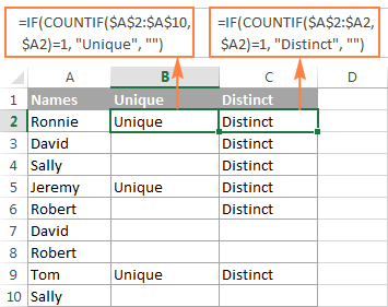
To find distinct or unique values in a list, use one of the following formulas, where A2 is the first and A10 is the last cell with data.
How to find unique values in Excel:
=IF(COUNTIF($A$2:$A$10, $A2)=1, "Unique", "")
How to get distinct values in Excel:
=IF(COUNTIF($A$2:$A2, $A2)=1, "Distinct", "")
In the distinct formula, there is just one small deviation in the second cell reference, which however makes a big difference:
Tip. If you'd like to search for unique values between 2 columns, i.e. find values that are present in one column but absent in another, then use the formula explained in How to compare 2 columns for differences.
Find unique / distinct rows in Excel
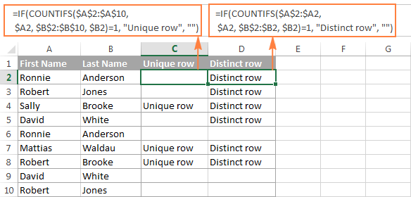
In a similar manner, you can find unique rows in your Excel table based on values in 2 or more columns. In this case, you need to use the COUNTIFS function instead of COUNTIF to evaluate the values in several columns (up to 127 range/criteria pairs can be evaluated in a single formula).
For example, to find unique or distinct names in the list, use the following formulas:
Formula to get unique rows:
=IF(COUNTIFS($A$2:$A$10, $A2, $B$2:$B$10, $B2)=1, "Unique row", "")
Formula to find distinct rows:
=IF(COUNTIFS($A$2:$A2, $A2, $B$2:$B2, $B2)=1, "Distinct row", "")
Find case-sensitive unique / distinct values in Excel
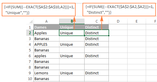
If you are working with a data set where case matters, you'd need a bit more trickier array formula.
Finding case-sensitive unique values:
=IF(SUM((--EXACT($A$2:$A$10,A2)))=1,"Unique","")
Finding case-sensitive distinct values:
=IF(SUM((--EXACT($A$2:$A2,$A2)))=1,"Distinct","")
Since both are array formulas, be sure to press Ctrl + Shift + Enter to complete them correctly.
When the unique or distinct values are found, you can easily filter, select and copy them as demonstrated below.
How to filter unique and distinct values in Excel
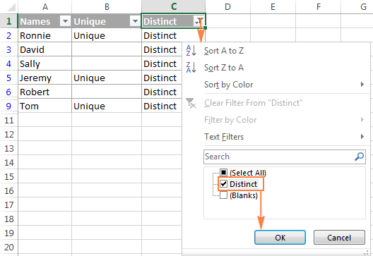
To view only unique or distinct values in the list, filter them out by performing the following steps.
- Apply one of the above formulas to identify unique / distinct values or rows.
- Select your data, and click the Filter button on the Data tab. Or, click Sort & Filter > Filter on the Home tab in the Editing group.
- Click the filtering arrow
 in the header of the column containing your formula and select the values you want to view:
How to select distinct / unique values
If you have a relatively small list of unique / distinct values, you can simply select it in the usual way using the mouse. If the filtered list contains hundreds or thousands of rows, you can use one of the following time-saving shortcuts.
To quickly select the unique or distinct list including column headers, filter unique values, click on any cell in the unique list, and then press Ctrl + A.
To select distinct or unique values without column headers, filter unique values, select the first cell with data, and press Ctrl + Shift + End to extend the selection to the last cell.
Tip. In some rare cases, mostly on very large workbooks, the above shortcuts may select both visible and invisible cells. To fix this, press either Ctrl + A or Ctrl + Shift + End first, and then press Alt + ; to select only visible cells, ignoring hidden rows.
If you have difficulties with remembering that many shortcuts, use this visual way: select the entire unique / distinct list, then go to the Home tab > Find & Select > Go to Special, and select Visible cells only.
Copy unique or distinct values to another location
To copy a list of unique values to another location, just do the following:
- Select the filtered values using the mouse or the above mentioned shortcuts.
- Press Ctrl + C to copy the selected values.
- Select the top-left cell in the destination range (it can be on the same or different sheet), and press Ctrl + V to paste the values.
How to highlight unique and distinct values in Excel
Whenever you need to highlight anything in Excel based on a certain condition, head right to the Conditional Formatting feature. More detailed information and examples follow below.
Highlight unique values in a column (built-in rule)
The fastest and easiest way to highlight unique values in Excel is to apply the inbuilt conditional formatting rule:
- Select the column of data where you want to highlight unique values.
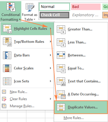
- On the Home tab, in the Styles group, click Conditional Formatting > Highlight Cells Rules >Duplicate Values...
- In the Duplicate Values dialog window, select Unique in the left-hand box, and choose the desired formatting in the right-hand box, then click OK.
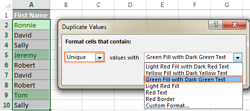
Tip. If you are not happy with any of the predefined formats, click Custom Format... (the last item in the drop-down list) and set the fill and/or font color to your liking.
As you see, highlighting unique values in Excel is the easiest task one could imagine. However, Excel's built-in rule works only for the items that appear in the list only once. If you need to highlight distinct values - unique and 1st duplicate occurrences - you will have to create your own rule based on a formula. You would also need to create a custom rule to highlight unique rows based on the values in one or more columns.
Highlight unique and distinct values in Excel (custom rule)
To highlight unique or distinct values in a column, select the data without a column header (you don't want the header to get highlighted, do you?), and create a conditional formatting rule with one of the following formulas.
Highlight unique values
To highlight the values that appear in a list just once, use the following formula:
=COUNTIF($A$2:$A$10,$A2)=1
Where A2 is the first and A10 is the last cell of the applied range.
Highlight distinct values
To highlight all different values in a column, i.e. unique values and 1st duplicate occurrences, go with the following formula:
=COUNTIF($A$2:$A2,$A2)=1
Where A2 is the top-most cell of the range.
How to create a formula based rule
To create a conditional formatting rule based on a formula, do the following:
- Go to the Home tab > Styles group, and click Conditional Formatting > New rule > Use a formula to determine which cells to format.
- Enter your formula on the Format values where this formula is true box.
- Click the Format... button and choose the fill color and/or font color you want.
- Finally, click the OK button to apply the rule.
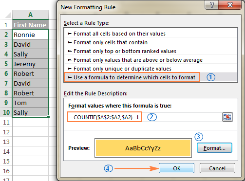
For more detailed steps with screenshots, please see the following tutorial: How to create an Excel conditional formatting rules based on another cell value.
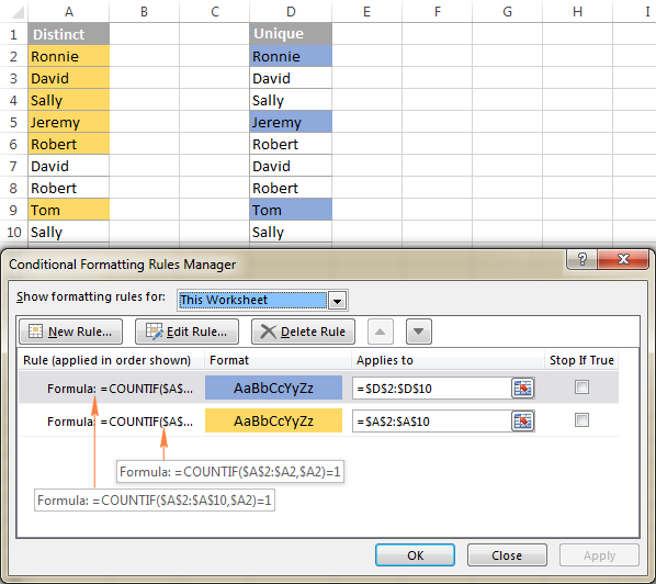
The below screenshot demonstrates both rules in action:
Highlight entire rows based on unique / distinct values in one column
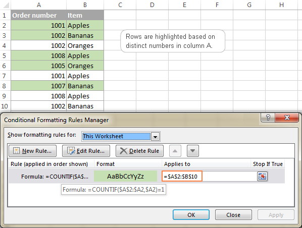
To highlight entire rows based on unique values in a specific column, use the formulas for unique and distinct values we used in the previous example, but apply your rule to the whole table rather than to a single column.
The following screenshot demonstrates the rule that highlights rows based on distinct numbers in column A:
How to highlight unique rows in Excel
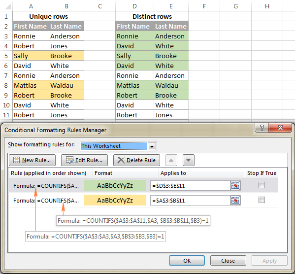
If you want to highlight rows based on the values in 2 or more columns, use the COUNTIFS function that allows specifying several criteria in a single formula.
Highlight unique rows
=COUNTIFS($A$2:$A$10,$A2, $B$2:$B$10,$B2)=1
Highlight distinct rows (unique + 1st duplicate occurrences)
=COUNTIFS($A$2:$A2,$A2,$B$2:$B2,$B2)=1
This is how you can find, filter and highlight distinct or unique values in Excel. To consolidate your knowledge, you can download the sample Find Unique Values workbook and reverse-engineer the formulas for better understanding.
Fast and easy way to find and highlight unique values in Excel
As you have just seen, Microsoft Excel provides quite a lot of useful features that can help you identify and highlight unique values in your worksheets. However, all those solutions can hardly be called intuitive and easy-to-use because they requires memorizing a handful of different formulas. Of course, it's no big deal for Excel professionals :) For those Excel users who want to save their time and effort, let me demonstrate a quick and straightforward way to find unique values in Excel.
In this final section of our today's tutorial, we are going to use our Duplicate Remover add-in for Excel. Please don't be confused by the tool's name. Apart from duplicate records, the add-in can perfectly handle unique and distinct entries, and you will make sure of it in a moment.
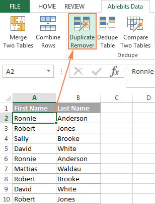
- Select any cell in a table where you want to find unique values and click the Duplicate Remover button on the Ablebits Data tab in the Dedupe group.
The wizard will run and the entire table will get selected automatically. So, just click Next to proceed to the next step.
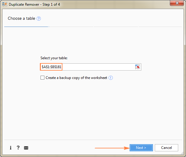
Tip. When using the add-in for the first time, it makes sense to check the Create a backup copy box, just in case.
- Depending on your goal, select one of the following options, and then click Next:
- Unique
- Unique +1st occurrences (distinct)
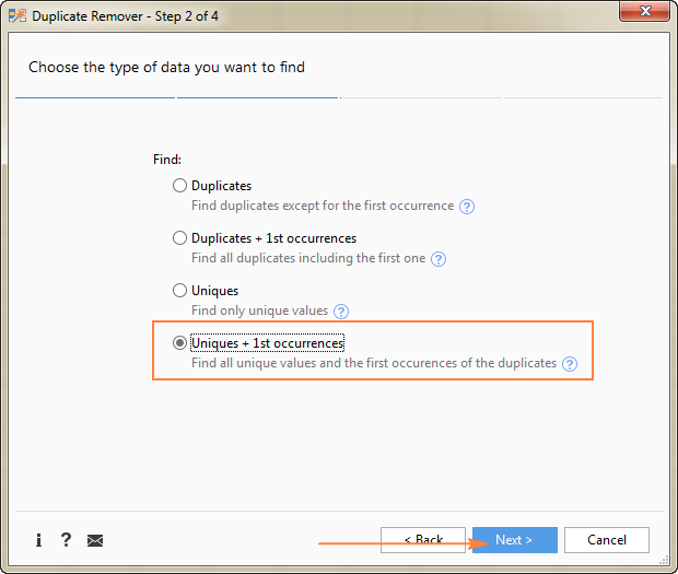
- Select one or more columns where you want to check the values.
In this example, we want to find unique names based on values in 2 columns (First name and Last name), therefore we select both.
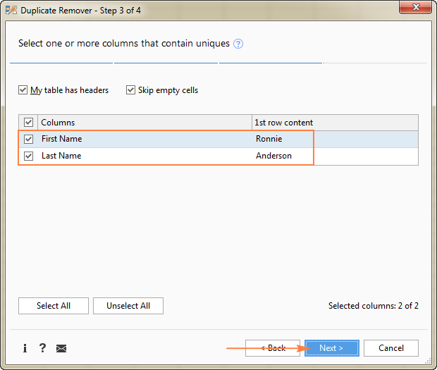
Tip. If your table has headers, be sure to select the My table has headers box. And if your table may have empty cells, make sure the Skip empty cells option is checked. Both options reside in the upper part of the dialog window and are usually selected by default.
- Choose one of the following actions to perform on the found values:
- Highlight unique values with color
- Select unique values
- Identify in a status column
- Copy to another location
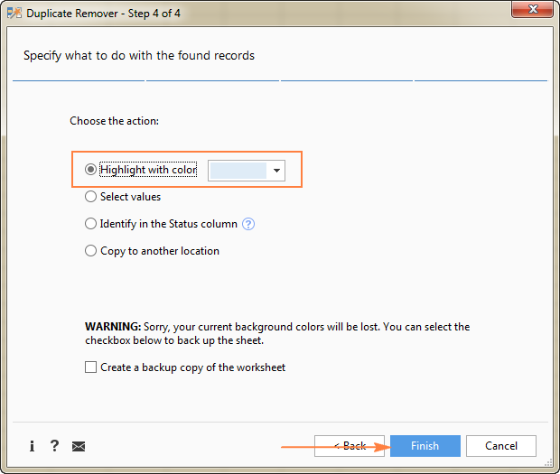
Click the Finish button, and get the result in seconds:
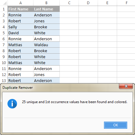
This is how you can find, select and highlight unique values in Excel using our Duplicate Remover add-in. It just couldn't be simpler, right?
If finding duplicate and unique values in Excel is a common part of your daily work, just try this dedupe tool and you will be amazed with the results! Duplicate Remover as well as our other time-saving tools are included with Ultimate Suite for Excel.
Available downloads
Find Unique Values - formula examples (.xlsx file)
Ultimate Suite - trial version (.exe file)
 by
by
46 comments
Hi, I have gone through the above article and its very useful.
based on this I tried to find out some solution, however I could not able to find out the solution.
I need to extract non unique data from the 2 different sheets.
In April 24, I have employee number 1001, 1002, 1003, 1004, 1005, 1006, 1007 and in May 2024 I have employee number 1001, 1002, 1003, 1004, 1007, 1008, 1009
I should get answer as new joinees in May 2024 - 1008, 1009 and Resigned in April - 1005, 1006
I tried solution with Unique with VSTAK, however I am not getting the correct solution. Request you to guide which formula I need to use to get the correct answer.
Thanks
Hi! Use COUNTIF function to determine matching and non-matching values in the two lists. The non-matching values will return 0. Then use FILTER function to show the non-matching values.
=FILTER(A2:A8,COUNTIF(B2:B8,A2:A8)=0)
=FILTER(B2:B8,COUNTIF(A2:A8,B2:B8)=0)
Here is the article that may be helpful to you: How to compare two columns in Excel for matches and differences
Thank you for reply, your solution is working perfectly
Thank you.
Imagine writing is entire guide and then finding out there's a unique function...
Hi James,
Firstly, at the time of writing this guide the UNIQUE function did not exist.
Secondly, the UNIQUE function extracts distinct values but does not label/identify them in the source list.
Thirdly, we have a guide for the UNIQUE function too :)
For the sub-topic "Find unique / distinct rows in Excel“ and the formula is "=IF(COUNTIFS($A$2:$A2, $A2, $B$2:$B2, $B2)=1, "Distinct row", "")"
If I want to this in Excel Power Query, how should I do it ?
Thanks
Please guide formulae for highlighted quantity available from total
Data
Total available
X 11
Y 15
Z 21
Product Quantity required
X 5
X 6
X 2
Y 8
Y 4
Y 7
Z 20
Z 15
Z 2
Hi!
Please clarify your problem or provide additional details to highlight exactly what you need. As it's currently written, it's hard to tell exactly what you're asking.
Hi
I have a transformation problem that I thought I might be able to solve using unique as on of the steps but might be on the complete wrong track. I have data that looks like this:
Id ItemsYes ItemsNo
1 230018;230019
2
3 231350;231351 231352
4 231350;231351;231352 231355
5
6 231350;231351
7 230019 230018
And need to look like this:
id 230018 230019 231350 231351 231352 231355
1 Yes Yes
2
3 Yes Yes No
4 Yes Yes Yes No
5
6 Yes Yes
7 No Yes
I thought to split the data in columns by the semicolon, then filter for unique numbers across all the rows and transpose these as new columns (then simple IF to populate Yes/No), but can work out how to get a single list of unique number from something this:
id ItemsYes.1 ItemsYes.2 ItemsYes.3 ItemsNo
1 230018 230019
2
3 231350 231351 231352
4 231350 231351 231352 231355
5
6 231350
7 230019 230018
Of course there could be an easier way altogether without the steps I'm thinking but would appreciate any suggestions
Hello!
Sorry, it's not quite clear what you are trying to achieve.
Yeah, I spaced it out but those all go taken out when I posted the comment. Also after reading more I know I mean distinct rather than unique.
Essentially the main ask is the bottom piece. I have multiple columns of 6-digit numbers (and empty cells) - The numbers in each row are unrelated so just I need a single column of distinct 6-digit numbers across all columns.
Hello!
To extract distinct values from a range, you can use an array formula.
=INDIRECT(TEXT(MIN(IF(($A$2:$C$9<>"")* (COUNTIF($E$1:E1,$A$2:$C$9)=0), ROW($2:$9)*100+COLUMN($A:$C),7^8)),"R0C00"),)&""
In this formula, the values are extracted from the range C2:E9.
Copy the formula down the column until there are empty cells.
Thanks Alexander! That works perfectly - I actually think I tried something like this but forget I needed to use an array formula.
Can you think of a way to get the same output where the raw data has delimiters instead of being in individual cells? e.g.
230018;230019
231350;231351
231350;231351;231352
231350;231351
Hello!
Divide this text into individual cells using the Text to columns tool or other methods described in this article.
I hope this will help.
Thank you. I was hoping to skip a step a rather large dataset but thank you for all you help, I'm finding the tools very useful.
Hi Have Two Columns- A and B
Column A - Has list of plant and column B- Has list of regions
I want to create Coulumn C in which all the regions related to a certain plant will come together.
Ex
Column A Column B Column C
Plant 100 India India,Denmark
Plant 200 France France
Plant 100 Denmark
is this possible? IF yes How
Any help will be appreciated
Hello!
You can find the examples and detailed instructions here: How to VLOOKUP multiple values in Excel with one or more criteria.
I hope it’ll be helpful.
I am trying to use =IF(COUNTIF($A$2:$A$10, $A2)=1, "Unique", "") to find out unique clients in Column A but I am not getting any result. I am using Excel 2010.
Hi!
You can see how this formula works in the first paragraph of this article. Copy the formula down the column.
I have four columns of numbers, I need to find which numbers are represented in column A that are not represented in B, C or D.
Hello!
I suggest writing the data that you will compare to two different files. Then use this instruction: How to compare two Excel files for differences
Recommend to use Duplicate Remover Toolkit for Excel
It is available as a part of our Ultimate Suite for Excel that you can install in a trial mode and check how it works for free.
If something is still unclear, please feel free to ask.
Dear I need solution of my following problem. As per rule a person can send transactions to max 15 distinct receiver in any given 90 days. I used countifs function, it works for me but the issue is that it doesnt configure distinct values, rather it count on base of total values.
Sender Receiver$ Transaction DatePrevious 90 DaysCount on receiver base
Ali Saad 130 01/01/2019 04/10/2018 1
Aslam Malik 200 18/01/2019 21/10/2018 1
Ali Saad 180 28/02/2019 01/12/2018 2
I use following formula
=COUNTIFS($A$2:$A$19,A4,$B$2:$B$19,B4,$D$2:$D$19,"="&E4)
u can see that Ali has sent only to Saad two time, but Saad is a distinct reciver, so answer at F4 should be 1. Please help
Hello!
Using your formula, I did not get the result you are writing about. But to remove the counting of duplicates, subtract from your formula the expression
=COUNTIFS($A$2:$A$19,A4,$B$2:$B$19,B4,$D$2:$D$19,"="&E4) - (COUNTIFS($A$2:$A$19,A4,$B$2:$B$19,B4)-1)
I hope my advice will help you solve your task.
IF DIA OF BAR IS 12 THE HOOK SIZE WILL BE 180
IF DIA OF BAR IS 14 THE HOOK SIZE WILL BE 220
IF DIA OF BAR IS 16 THE HOOK SIZE WILL BE 250
IF DIA OF BAR IS 20 THE HOOK SIZE WILL BE 300
IF DIA OF BAR IS 25 THE HOOK SIZE WILL BE 400
IF DIA OF BAR IS 32 THE HOOK SIZE WILL BE 500
IF I PUT DIA IN TABLE CELL THE CONNECTING TABLE CELL SHOULD GIVE THE HOOK SIZE FOR MY CALCULAITON SHEET
Hello Mohammed!
Use the IF function with several conditions. Read more in this article.
Greetings,
Thank you for publishing a post which is both useful and informative.
I am using the following formula from above to identify distinct values in a column: =IF(COUNTIF($A$2:$A2, $A2)=1, "Distinct", "")
Is it possible to use structured references with this formula?
If not, can you point me to an alternative formula that does allow the use of structured references while accomplishing the same function?
Thank you for your time,
Loch
Hello Loch!
I think that it is not possible to use structured references in your case. A named range or structured references mean that you have a fixed data range which you’ve given some name. In your case the size of the range changes in each new row.
Alas, that was my fear. Thanks for the reply.
Wondering how can this be added to an arrayformula?
=IF(COUNTIF($A$2:$A$10, $A2)=1, "Unique", "")
Actually wanted to understand how to add the ARRAYFORMULA for the distinct formula (not the unique):
=IF(COUNTIF($A$2:$A2, $A2)=1, "Distinct", "")
Hi Lian,
That does not need to be an array formula, it works as a regular formula just fine. Simply, enter it in any empty cell in row 2, press Enter, and then drag the formula down to as many cells as needed.
Would like to sort a column, and alternately highlight the rows according to the value that has the same value from the sorted column. For example, sort the first name, and highlight the whole rows of those with "Art", change color to "Bob", change color back to "Charlie", etc.
Hi,
How do I count duplicate values as 1 only?
I want to count a column containing unique values but have duplicates count as 1.
I need to be able to apply a distinct filter AFTER I filter many other columns. Is this possible?
i want data this type
Company Cost
Company Cost
Angel South 990
Angel South 4334
Angel South 3232
Arnold Inc 1200
Arnold Inc 1200
Edison LLC 1750
Edison LLC 3233
Edison LLC 3232
Lloyds 1200
Parker 1200
Parker 3233
Southern Best 1825
Southern Best 4334
Southern Best 1200
Angel South 990 4334 3232
Arnold Inc 1200 1200
Edison LLC 1750 3233 3232
Lloyds
Parker 1200 3233
Southern Best 1825 4334 1200
left side data converter into right side data in excel
so please tell me any suggestion about my prob
i want data this type
Company Cost
Angel South 990 Angel South 990 4334 3232
Angel South 4334 Arnold Inc 1200 1200
Angel South 3232 Edison LLC 1750 3233 3232
Arnold Inc 1200 Lloyds 1200
Arnold Inc 1200 Parker 1200 3233
Edison LLC 1750 Southern Best 1825 4334 1200
Edison LLC 3233
Edison LLC 3232
Lloyds 1200
Parker 1200
Parker 3233
Southern Best 1825
Southern Best 4334
Southern Best 1200
left side data converter into right side data in excel
so please tell me any suggestion about my prob
Hello People,
I have a huge data coming from a call center. I need to retrieve unique mobile numbers from a particular column. Can somebody help me out please.
Kindly find a set of data from the column. Hope it might help in jotting the right path/formula.
8247487020
9490574653
9966660233
8374821105
7095833350
9133451069
9392957677
7095833350
9392957677
7095606291
7760527557
9133451069
9392861610
9948382932
9603363044
9704420942
9849328753
7095833350
9640752564
9640752564
9603363044
9247321093
7095833350
7095833350
9603363044
9676244615
8374821105
6304424104
9394782188
9000565415
9394782188
Hello, Prashanth.
If your task is to find unique values in your column, our Duplicate Remover can solve it at a glance. The add-in helps you find unique values in your workbook and highlight/copy/move them if necessary.
Hi,
I have a huge worksheet were there are event ids.. From that i need to select unique one and then end up to the counts as how many evemts are there.
Eg:
100 event id
Out of 100 50 are duplicate
Will remain 50
So the count 50 i want as a end result
Regards,
Bhavika Ravani
Bhavika:
The answer to your question is more complicated than you may realize. Rather than just providing you with a formula to try and answer your question, I think it will benefit you much more if you would take a look at this article and the other articles linked therein dealing with counting distinct values starting here:
https://www.ablebits.com/office-addins-blog/count-distinct-unique-values-excel/#count-distinct-text
Hi team,
I have multiple excel file run out of macro. So if i want to use any formulae i m unablw to use.
Is there ny way data gets auto pulled to another file n distinct values are auto counted if designed in VBA
regards,
Bhavika Ravani
Sir,
Pls give solution. Particular one cell in more data value (exp: 45,56,45,56)how to find duplicate value in one cell.
Dear Sevtlana,
This is my second request. Sorry. I am just trying to ask some help regarding a formula a for a cell using conditional formatting, i badly need this for my training matrix which covers different trainings and different expiry dates.
Training dates that will highlight if it will expire in 1,2,3 years
1 yr ( example 01-Aug-2016 will expire in 01-Aug-2017 onward ) and ( 1 year before the current date) highlighting in red with white font
2 yr ( example 01-Aug-2016 will expire in 01-Aug-2018 onward ) and ( 2 year before the current date) highlighting in red with white font
3 yr ( example 01-Aug-2016 will expire in 01-Aug-2019 onward ) and ( 3 years before the current date) highlighting in red with white font
And it highlight on different color if cell value is blank/empty
Please help me on this. i have been trying to ask help to all my friends but no one knows.
Thanks and God bless
Carwell
Dear Carwell,
You can create a few conditional formatting rules with the following formulas:
Expire in 1 yr: =DATEDIF($A1, TODAY(), "y")<=1
Expire in 2 yr: =DATEDIF($A1, TODAY(), "y")<=2
Expire in 3 yr: =DATEDIF($A1, TODAY(), "y")<=3
To highlight blank cells, use this formula: =$A1=""
Where A1 is the topmost cell with a date.
The detailed instructions on conditionally formatting dates can be found here:
https://www.ablebits.com/office-addins-blog/excel-conditional-formatting-dates/
I need help with the following =If(B2:B11)="Pass","Completed" it works if I just us B2 but when I want to see if "Pass" is in each field that is when I get an error.
Hello Rhonda,
If you want to show "Completed" in each row, if a cell in column B in that row is "Pass", you can enter the following formula in row 2, and then copy it down to row 11:
=IF(B2="Pass","Completed", "")
If you want to show "Completed" if all 10 cells (B2:B11) contain "pass", then use this formula:
=IF(COUNTIF(B2:B11, "pass")=10, "completed", "")