The tutorial introduces a new Excel 365 dynamic array function that can expand an array to the desired dimensions with a value of your choosing.
Want to increase an array to a specified number of rows or columns so that all similar arrays in your worksheet have the same size? In Excel 365, that can be done with one simple formula. Meet the brand-new EXPAND function that can grow an array to any dimensions you set.
Excel EXPAND function
The EXPAND function in Excel is designed to pad an array with a value of your choice to the specified row and column dimensions.
The syntax includes the following arguments:
Where:
Array (required) - the original array.
Rows (optional) - the number of rows in the returned array. If omitted, new rows are not added, and the columns argument must be set.
Columns (optional) - the number of columns in the returned array. If omitted, new columns are not added, and the rows argument must be set.
Pad_with - the value to fill new cells with. If omitted, defaults to #N/A.
Tip. To remove unwanted rows or columns from an array, use the DROP function.
EXPAND function availability
Currently, the EXPAND function is available in Excel for Microsoft 365 (Windows and Mac) and Excel for the web.
How to use the EXPAND function in Excel
To increase an array to the desired size, construct an EXPAND formula in this way:
- For array, supply a range of cells or an array of values returned by another formula.
- For rows and columns, provide positive numbers that are greater than the number of rows and columns in the original array. Note that these arguments define the dimensions of the resulting array, not the number of rows or columns to add. In each particular formula, either rows or columns must be set. The omitted argument defaults to the corresponding dimension (rows or columns) of the source array.
- For pad_with, specify the value to populate the new cells added to the array. If it's a text value, enclose it in double quotes. If it's a numeric value, use it without quotation marks. If not provided, the new cells will be padded with the #N/A error.
Being a dynamic array function, EXPAND needs to be entered only in one cell, and it automatically spills the results into as many cells as specified in the rows and columns arguments.
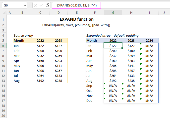
For example, to expand the array C6:D13 to 12 rows and 3 columns, the formula is:
=EXPAND(C6:D13, 12, 3)
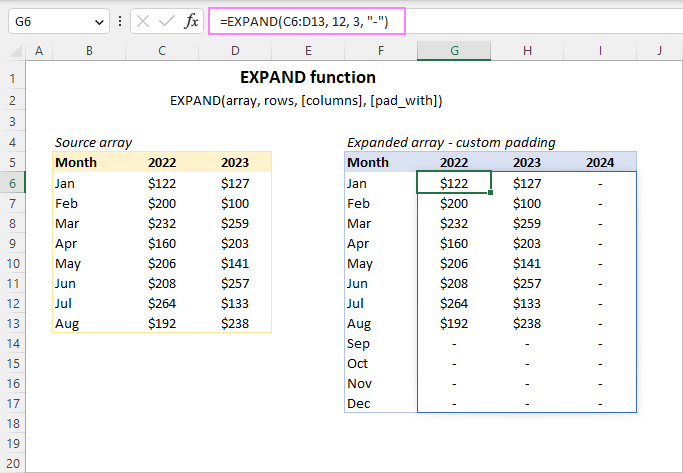
As the pad_with argument is not set, the above formula will pad the newly added cells with the #N/A error. To change the default behavior, supply any value you want for the pad_with argument. For example, you can pad the new array values with a hyphen:
=EXPAND(C6:D13, 12, 3, "-")
Below you will find a few more examples of using the EXPAND function in Excel to grow an array in a specific direction.
Expand array to a certain number of rows
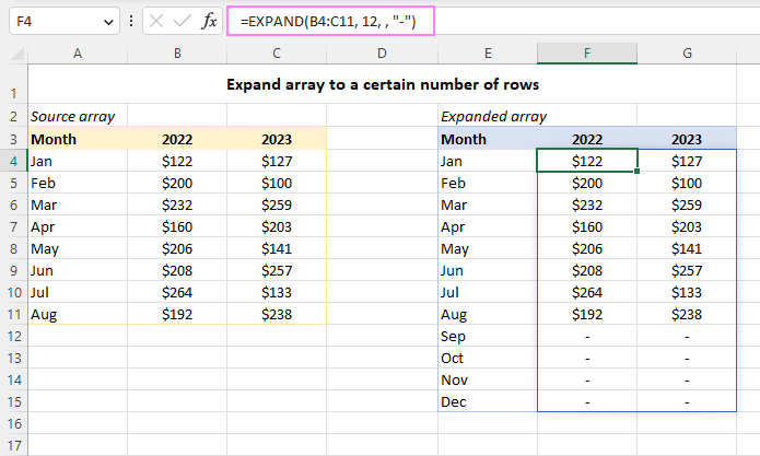
To extend an array down to the desired number of rows, define the rows argument and omit columns.
For instance, to increase the initial array to a total of 12 rows, use this formula:
=EXPAND(C6:D13, 12, , "-")
Because columns should not be extended, we type a comma after rows, and after the comma enter the padding value.
Expand array to a certain number of columns
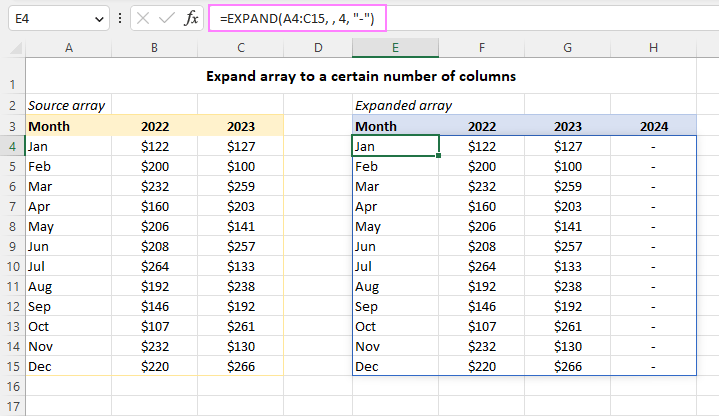
To add more columns to an array, define the columns argument and omit rows.
For example, here's how you can extend the source array to the right, so it has a total of 4 columns:
=EXPAND(A4:C15, , 4, "-")
How to expand an array left and up
The EXPAND function is designed to extend an array right and down. To add cells to the left and above of the source array, you will have to work out your own solution.
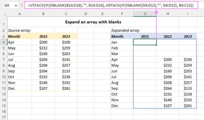
Suppose you have an array of values in B4:C12. You aim to add 3 rows above and 1 column to the left of the original array. To better understand the mechanics, we'll first perform each task individually, and then put all the pieces together.
Add columns to left
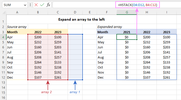
To extend the array horizontally, you can use the HSTACK function to append a given number of empty columns to the left of your array. In this example, we add 1 blank column using this formula:
=HSTACK(D4:D12, B4:C12)
Notice that an empty array that you stack (D4:D12) should have the same number of rows as the source array and should be supplied first in the formula. As a result, a column of zero values is added to the left of the original array.
Add rows above
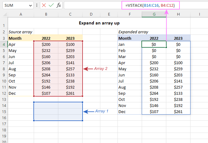
To expand the array vertically, leverage the VSTACK function to place a certain number of empty rows above the first row of your original array.
In our case, the following two ranges with the same number of columns are stacked, an empty array coming first:
=VSTACK(B14:C16, B4:C12)
In the result, 3 rows with zero values are added to the top of the initial array.
Add rows above and columns to left
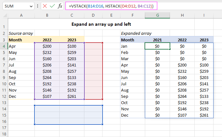
To expand an array vertically and horizontally, nest the VSTACK and HSTACK function one into the other. In our case, the formula takes this form:
=VSTACK(B14:D16, HSTACK(D4:D12, B4:C12))
And produces this result:
Pad an array up and left with custom value
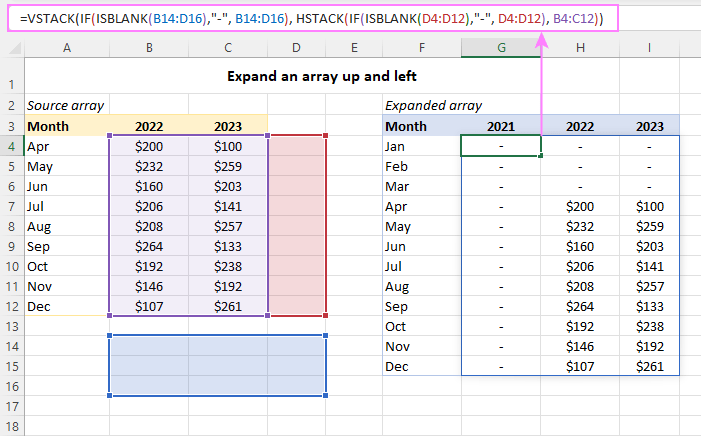
By default, the VSTACK and HSTACK functions return zeros instead of blank cells. To pad the new cells with a custom value, nest a combination of IF and ISBLANK within each stack function, which will replace blanks with the value you specify.
For example, to get the new cells padded with a hyphen, the formula is:
=VSTACK(IF(ISBLANK(B14:D16),"-", B14:D16), HSTACK(IF(ISBLANK(D4:D12),"-", D4:D12), B4:C12))
To extend an array with blank cells, use this formula:
=VSTACK(IF(ISBLANK(B14:D16),"", B14:D16), HSTACK(IF(ISBLANK(D4:D12),"", D4:D12), B4:C12))
Split strings and expand arrays
This example shows how to use the EXPAND and TEXTSPLIT functions together to split a text string by a specific delimiter in individual columns, and then grow the final array to the desired size.
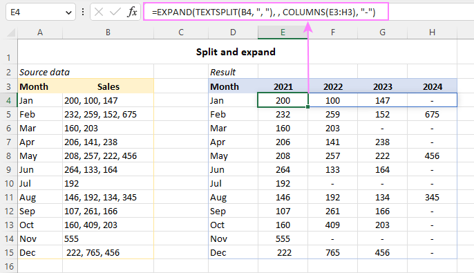
Let's say you have a column of strings like column B in the image below. Each string has several values separated with a particular delimiter (a comma and a space in our case). Your goal is to split each string into separate cells, so that all the resulting arrays have the same number of columns.
To accomplish the task, enter this formula in E4:
=EXPAND(TEXTSPLIT(B4, ", "), , COLUMNS(E3:H3), "-")
In this formula:
- TEXTSPLIT separates the values in B4 using a comma and a space (", ") as the delimiter.
- COLUMNS computes the number of columns in the output array.
- EXPAND extends the returned array to the right padding missing values with hyphens ("-").
Drag the formula down through E15 and you'll get this result:
EXPAND function not working
If the EXPAND function works incorrectly in your Excel or throws an error, the following tips will help you pin down the cause and fix it.
#VALUE! error
Occurs if the value used for the rows or columns argument is less than the total number of rows or columns of the source array.
#N/A error
Appears in padded cells if the pad_with argument is not set.
#NAME? error
Occurs if either the function's name is misspelled or EXPAND is not available in your Excel version. Currently, it's only supported in Excel 365 and Excel for the web. More details can be found in Fixing the #NAME error in Excel.
#SPILL! error
Occurs when there are not enough empty cells to output the expanded array. In most situations, clearing the obstructing cells fixes the error at once. For more information, please see How to fix #SPILL! error in Excel.
That's how to use the EXPAND function in Excel to extend an array to as many rows and columns as your business logic requires. I thank you for reading and hope to see you on our blog next week!
Practice workbook for download
Excel EXPAND formula - examples (.xlsx file)
 by
by
10 comments
Hi,
this is nicely explained, thank you for your guidance.
Can we add Unique function in argument of [pad_with] in Expand formula. I am getting error while trying this function.
Hi! Unfortunately, this information is not enough to give you any advice. Please specify what you were trying to find, what formula you used and what problem or error occurred.
Thank your for your quick reply,
I want to repeat the unique data multiple times as below.
EXPAND(UNIQUE(Data!D7:F134),COUNTA(UNIQUE(Data!D7:F134))/3*COUNTA(D1:H1),3,"Unique data to be appear")
in above formula I have updated the "(UNIQUE(Data!D7:F134)" formula [pad_with] argument.
I could have shared a sample file if I had the upload option.
Hi! If you read the article above carefully, with the EXPAND function you cannot repeat your data. You can extend the data range and fill new cells with some values. In your case, the result of the expression COUNTA(UNIQUE(Data!D7:F134))/3*COUNTA(D1:H1) must be greater than 127.
Thank you, the total rows of unique data is 16 and it has been repeated 5 times and it extended to 80 rows.
I understand that different values cannot be update in [pad_with] argument. Is there any other way to achieve our requirement.
I have the below list, and unique data is Administration, HR, Finance. In Expanded data this unique data need to updated with multiple times.
Administration
HR
Finance
Finance
HR
Administration
Hi! To merge multiple arrays, try the VSTACK function. Try the following formula:
=VSTACK(UNIQUE(Data!D7:F134),UNIQUE(Data!D7:F134),UNIQUE(Data!D7:F134),UNIQUE(Data!D7:F134),UNIQUE(Data!D7:F134))
Thank you very much for solution, its working when I want to repeat only few times, sometimes I want this unique data 50 - 60 times. Is there any possibilities to reflect multiple time with adding any other condition.
Hi! To copy a range of cells multiple times, use Paste Special. Copy values, select the range to insert, select Paste Special - Insert values.
Thank you very much.
The ultmate functionality of EXPAND is slghtly mysterious. In your first example, Expand array to a certain number of rows, you can write
=IF(C6:D17=0,"",C6:C17)
And thus be able to enter data for the remaining months in the new array.