In this tutorial, we'll take an in-depth look at the Excel 365 function named CHOOSEROWS and its practical uses.
Suppose you have an Excel worksheet with hundreds of rows from which you want to extract some specific ones, say, all odd or even rows, the first 5 or the last 10 rows, etc. Do you already feel annoyed at the thought of copying and pasting the data manually or writing a VBA code to automate the task? Don't worry! All is much simpler than it seems. Just use the new dynamic array CHOOSEROWS function.
Excel CHOOSEROWS function
The CHOOSEROWS function in Excel is used to extract the specified rows from an array or range.
The syntax is as follows:
Where:
Array (required) - the source array.
Row_num1 (required) - an integer representing the numeric index of the first row to return.
Row_num2, … (optional) - index numbers of additional rows to return.
Here's how the CHOOSEROWS function works in Excel 365:
The CHOOSEROWS function is only available in Excel for Microsoft 365 (Windows and Mac) and Excel for the web. Tip. To get certain columns from a range or array, use the CHOOSECOLS function.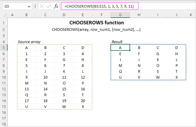
CHOOSEROWS function availability
How to use CHOOSEROWS function in Excel
To pull particular rows from a given array, construct a CHOOSEROWS formula in this way:
- For array, you can supply a range of cells or an array of values driven by another formula.
- For row_num, provide a positive or negative integer indicating which row to return. A positive number retrieves a corresponding row from the start of the array, a negative number - from the end of the array. Multiple row numbers can be provided individually in separate arguments or in one argument in the form of an array constant.
As a Excel dynamic array function, CHOOSEROWS handles arrays natively. You enter the formula in the upper-left cell of the destination range, and it automatically spills into as many columns and rows as needed. The result is a single dynamic array, also known as a spill range.
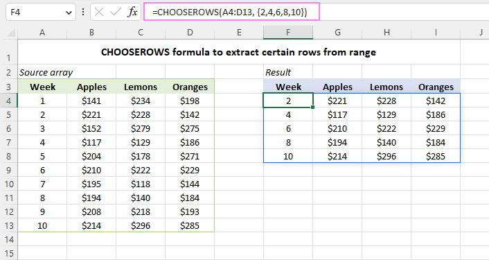
For example, to get rows 2, 4, 6, 8 and 10 from the range A4:D13, the formula is:
=CHOOSEROWS(A4:D13, 2, 4, 6, 8, 10)
Alternatively, you can use an array constant such as {2,4,6,8,10} or {2;4;6;8;10} to specify the desired rows:
=CHOOSEROWS(A4:D13, {2,4,6,8,10})
Or
=CHOOSEROWS(A4:D13, {2;4;6;8;10})
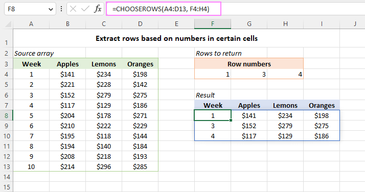
Another way to supply the row numbers is entering them in separate cells, and then using either the individual cell references for several row_num arguments or a range reference for a single row_num argument.
For example:
=CHOOSEROWS(A4:D13, F4, G4, H4)
=CHOOSEROWS(A4:D13, F4:H4)
An advantage of this approach is that it lets you extract any other rows by simply changing the numbers in the predefined cells without editing the formula itself.
Below we will discuss a few more CHOOSEROWS formula examples to handle more specific use cases.
Return rows from the end of an array
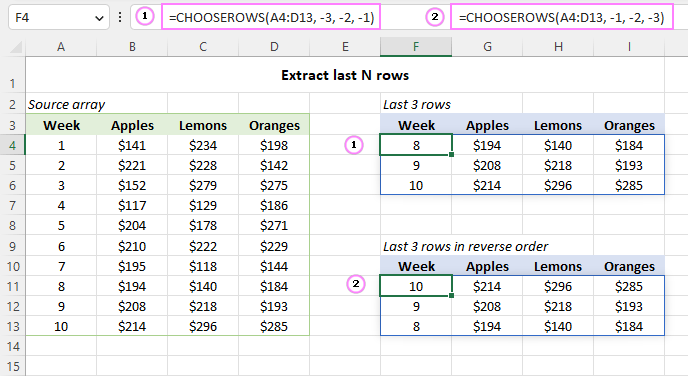
To quickly get the last N rows from a range, provide negative numbers for the row_num arguments. This will force the function to count rows from the end of the array.
For instance, to get the last 3 row from the range A4:D13, use this formula:
=CHOOSEROWS(A4:D13, -3, -2, -1)
The result will be a 3-row array where the rows appear in the same ordered as in the referred range.
To return the last 3 rows in the reverse order, from bottom to top, change the order of the row_num arguments like this:
=CHOOSEROWS(A4:D13, -1, -2, -3)
Extract every other row from an array in Excel
To get every other row from a given range, use CHOOSEROWS in combination with a few other functions. The formula will slightly vary depending on whether you are extracting odd or even rows.
To return odd rows such as 1, 3, 5, … the formula takes this form:
=CHOOSEROWS(A4:D13, SEQUENCE(ROUNDUP(ROWS(A4:D13)/2, 0), 1, 1, 2))
To return even rows such as 2, 4, 6, … the formula goes as follows:
=CHOOSEROWS(A4:D13, SEQUENCE(ROUNDDOWN(ROWS(A4:D13)/2, 0), 1, 2, 2))
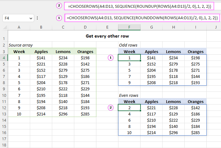
How this formula works:
In essence, the CHOOSEROWS function returns rows based on an array of sequential odd or even numbers generated by the SEQUENCE function. A detailed formula break-down follows below.
Firstly, you determine how many rows to return. For this, you employ the ROWS function to get the total number of rows in the referenced array, which you divide by 2, and then round the quotient upward or downward to the integer with the help of ROUNDUP or ROUNDDOWN. As this number will later be served to the rows argument of SEQUENCE, rounding is needed to get an integer in case the source range contains an odd number of rows.
As our source range has an even number of rows (10) that is exactly divided by 2, both ROUNDUP(10/2, 0) and ROUNDDOWN(10/2, 0) return the same result, which is 5.
The returned number is served to the SEQUENCE function.
For odd rows:
SEQUENCE(5, 1, 1, 2)
For even rows:
SEQUENCE(5, 1, 2, 2)
The SEQUENCE formula above produces an array of numbers consisting of 5 rows and 1 column, starting at 1 for odd rows (at 2 for even rows), and incremented by 2.
For odd rows, we get this array:
{1;3;5;7;9}
For even rows, we get this one:
{2;4;6;8;10}
The generated array goes to the row_num1 argument of CHOOSEROWS, and you get the desired result:
=CHOOSEROWS(A4:D13, {1;3;5;7;9})
Reverse the order of rows in an array
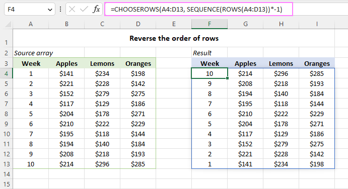
To flip an array vertically from top to bottom, you can also use the CHOOSEROWS and SEQUENCE functions together. For example:
=CHOOSEROWS(A4:D13, SEQUENCE(ROWS(A4:D13))*-1)
In this formula, we set only the first argument (rows) of SEQUENCE, which equals the total number of rows in the initial array ROWS(A4:D13). The omitted arguments (columns, start, step) default to 1. As a result, SEQUENCE produces an array of sequential numbers such as 1, 2, 3, …, n, where n is the last row in the source array. To make CHOOSEROWS count rows in the down-up direction, the generated sequence is multiplied by -1, so the row_num argument gets an array of negative numbers such as {-1;-2;-3;-4;-5;-6;-7;-8;-9;-10}.
As a result, the order of items in each column is changed from top to bottom:
Extract rows from multiple arrays
To get specific rows from two or more non-contiguous ranges, you first combine them using the VSTACK function, and then pass the merged range to CHOOSEROWS.
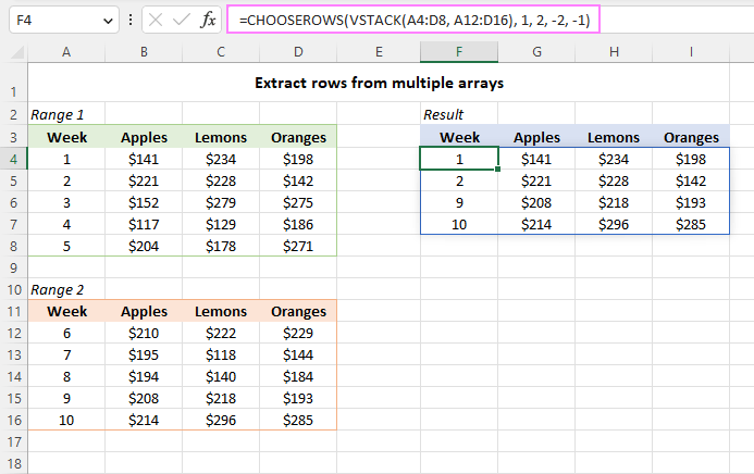
For example, to extract the first two rows from the range A4:D8 and the last two rows from the range A12:D16, use this formula:
=CHOOSEROWS(VSTACK(A4:D8, A12:D16), 1, 2, -2, -1)
Get rows based on a string containing row numbers
This example shows how to return particular rows by extracting the numbers from an alpha-numeric string.
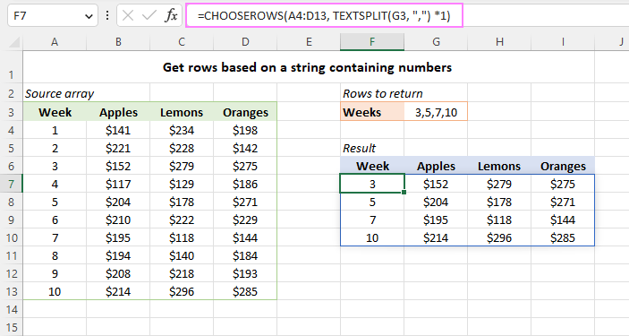
Suppose you have comma-separated numbers in cell G3 listing the rows of interest. To extract the row numbers from a string, use the TEXTSPLIT function that can split a text string by a given delimiter (comma in our case):
=TEXTSPLIT(G3, ",")
The result is an array of text values such as {"3","5","7","10"}. To convert it to an array of numbers, perform any math operation that does not change the values, say +0 or *1.
=TEXTSPLIT(G3, ",") *1
This produces the numeric array constant {3,5,7,10} that the CHOOSEROWS function needs, so you embed the TEXTSPLIT formula in the 2nd argument:
=CHOOSEROWS(A4:D13, TEXTSPLIT(G3, ",") *1)
As a result, all the specified rows are returned as a single array:
CHOOSEROWS function not working
If the CHOOSEROWS formula results in an error, it's most likely to be one of these reasons.
#VALUE! error
Occurs if the absolute value of any row_num argument is zero or higher than the total number of rows in the array.
#NAME? error
Occurs if the function's name is misspelled or the function is not supported in your Excel. Currently, CHOOSEROWS is only available in Excel 365 and Excel for the web. For more details, read How to fix #NAME error in Excel.
#SPILL! error
Occurs when there are not enough blank cells to fill with the results. To fix it, just clear the obstructing cells. For more information, please see Excel #SPILL! error.
That's how to use the CHOOSEROWS function in Excel to return particular rows from a range or array. Thank you for reading and I hope to see you on our blog next week!
Practice workbook for download
Excel CHOOSEROWS formula - examples (.xlsx file)
 by
by
4 comments
I have two tabs; Projects, which has headers in row 9 and data below this row, and Dates, which has headers in row 1 and data below this row.
In the Projects tab, from row 10 onwards, I have a row per project and 5 sets of 2 columns that contain formulae and evaluate to a date, or to a blank. This forms the criteria for which the next part is based on. The references for these sets of columns are | X & Y | AH & AI | AO & AP | AU & AV | AW & AZ |
In the same tab, I have 3 columns of dynamic data: Project Name(F), Project Code(G), Project Location(H). I need to extract values in rows from these 3 columns, into columns Project Name(A), Project Code(B), Project Location(C) respectively, in another tab (Dates), if certain criteria are met.
Criteria: in the Projects tab, in the first row containing data (row 10¬), if only one of either dates in the 1st set of dates (columns X & Y) are missing, then extract data from row 10, columns F, G & H to columns A,B & C in the Dates tab and extract the date that is present in either column to column F (Deadline) in the Dates tab, otherwise check the next set of dates in the same row. If the 2nd set of dates (columns AH & AI) only has either date missing, then extract the data from row 10, columns F, G & H and the date, etc., until all 5 sets of dates are checked for a row. Repeat this for all rows that contain data in columns F, G & H.
This will mean that every project and its row in the Project tab, will potentially generate 5 rows of data in the Dates tab (depending on if the criteria is met). E.g., in the Projects tab in row 10, there are dates in columns X, AH, AI, AP, & AV. The date columns Y, AO, AU, AW & AZ are empty.
The cells will therefore return the following values:
Dates (A2) – Projects (F10)
Dates (A3) – Projects (F10)
Dates (A4) – Projects (F10)
Dates (B2) – Projects (G10)
Dates (B3) – Projects (G10)
Dates (B4) – Projects (G10)
Dates (C2) – Projects (H10)
Dates (C3) – Projects (H10)
Dates (C4) – Projects (H10)
Dates (F2) – Projects (X10)
Dates (F3) – Projects (AP10)
Dates (F4) – Projects (AV10)
I am using the formula as below in the Dates tab to return values if the criteria is met, and a blanks if not.
=IF(OR(AND(‘Projects’!X$6="",’Projects’!Y$6=""),AND(ISNUMBER(‘Projects’!X$6),ISNUMBER(‘Projects’!Y$6))),"",’Projects’!$F$6)
I have two problems with this formula though; one is that when the formula was dragged down, parts had to be manually edited so that the correct values are returned (because each row down in the Dates tab won’t necessarily retrieve data from the next row down in the Projects tab, it could be from the same row). The other problem I have is that using this formula will result in several rows that return no data due to the criteria not being met.
I then came across this article, and using the CHOOSEROWS function is more efficient than formulae in each column, however I’ll still have the same two problems above.
To further complicate this, I will potentially have more sets of dates added to the Projects tab in the future, and need the formula to easily accommodate the extra sets of dates, without having to manually amend parts of the formula that have been copied down (there will be several hundreds of rows in the Projects tab).
Is there one formula that could do it all?
Hi! Despite the very detailed description, it is difficult to understand the calculations without seeing your complex data. But if there is no exact matching between table rows, it is impossible to copy a formula down a column without errors.
Thank you for the reply Alexander, I had a feeling you'd say it's impossible for the formula to work when copied down but thought I'd check with an expert. I have solved this now, and decided that when I need to amend the formulae to accommodate more sets of columns with dates, I will use VBA instead of manually writing formula for each row.
I literally love the blogs of ablebits on excel♥️.
I too need help in ms word & Power Point.
Please if you know a website for these two then please tell me. I checked out few websites but there are no screenshots not proper explanations.
I request the maintainers & owners of ablebits to please guide me.
Thanks and lots of love.