The tutorial shows how to safely merge rows in Excel in 4 different ways: merge multiple rows without losing data, combine duplicate rows, repeatedly merge blocks of rows, and copy matching rows from another table based on one or more common columns.
Merging rows in Excel is one of the most common tasks that all of us need to perform every now and then. The problem is that Microsoft Excel does not provide a reliable tool to do this. For example, if you try to combine two or more rows using the built-in Merge & Center button, you will end up with the following error message:
"The selection contains multiple data values. Merging into one cell will keep the upper-left most data only."

Clicking OK will merge the cells but only keep the value of the first cell, all other data will be gone. So, obviously we need a better solution. This article describes several methods that will let you merge multiple rows in Excel without losing any data.
How to merge rows in Excel without losing data
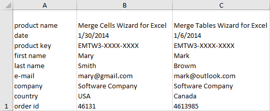
The task: you have a database where each row contains certain details such as product name, product key, customer name and so on. What we want is to combine all the rows related to a particular order like shown below:
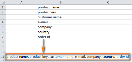
There are two ways to achieve the desired result:
Merge multiple rows using formulas
To joint the values from several cells into one, you can use either the CONCATENATE function or concatenation operator (&). In Excel 2016 and higher, you can also use the CONCAT function. Any way, you supply cells as references and type the desired delimiters in-between.
Merge rows and separate the values with comma and space:
=CONCATENATE(A1,", ",A2,", ",A3)
=A1&", "&A2&", "&A3
Merge rows with spaces between the data:
=CONCATENATE(A1," ",A2," ",A3)
=A1&" "&A2&" "&A3
Combine rows and separate the values with commas without spaces:
=CONCATENATE(A1,A2,A3)
=A1&","&A2&","&A3
In practice, you may often need to concatenate more cells, so your real-life formula is likely to be a bit longer:
=CONCATENATE(A1,", ",A2,", ",A3,", ",A4,", ",A5,", ",A6,", ",A7,", ",A8)
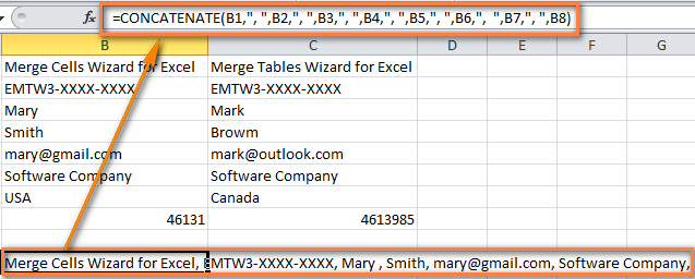
Now you have several rows of data merged into one row. But your combined rows are formulas. To convert them to values, use the Paste Special feature as described in How to replace formulas with their values in Excel.
Combine rows in Excel with Merge Cells add-in
The Merge Cells add-in is a multi-purpose tool for joining cells in Excel that can merge individual cells as well as entire rows or columns. And most importantly, this tool keeps all the data even if the selection contains multiple values.
To merge two or more rows into one, here's what you need to do:
- Select the range of cells where you want to merge rows.
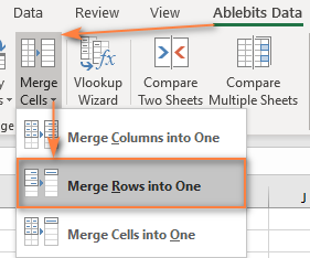
- Go to the Ablebits Data tab > Merge group, click the Merge Cells arrow, and then click Merge Rows into One.
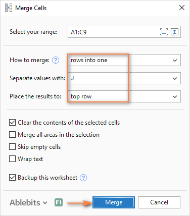
- This will open the Merge Cells dialog box with the preselected settings that work fine in most cases. In this example, we only change the separator from the default space to line break, as shown in the screenshot below:
- Click the Merge button and observe the perfectly merged rows of data separated with line breaks:
How to combine duplicate rows into one (keeping unique values only)
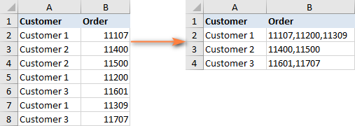
The task: you have some Excel database with a few thousand entries. The values in one column are essentially the same while data in other columns are different. Your goal is to combine data from duplicate rows based on a certain column, making a comma separated list. Additionally, you may want to merge unique values only, omitting duplicates and skipping empty cells.
The screenshot below shows what we are trying to achieve.
The prospect of finding and merging duplicate rows manually is definitely something you'd want to avoid. Meet the Merge Duplicates add-in that turns this time-consuming and cumbersome chore into a quick 4-steps process.
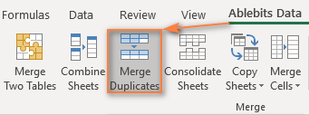
- Select the duplicate rows you want to merge and run the Merge Duplicates wizard by clicking its button on the ribbon.
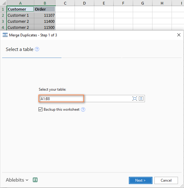
- Make sure your table is selected correctly and click Next. It is wise to keep the Create a backup copy option checked, especially if you are using the add-in for the first time.
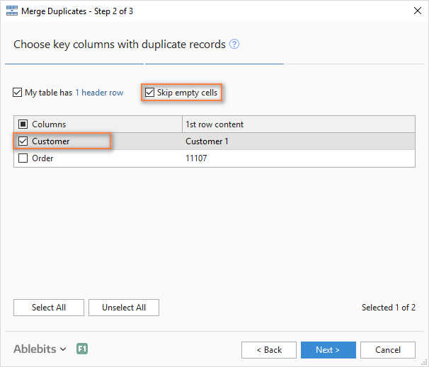
- Select the key column to check for duplicates. In this example, we select the Customer column because we want to combine rows based on customer name.
If you want to skip empty cells, be sure to select this option and click Next.
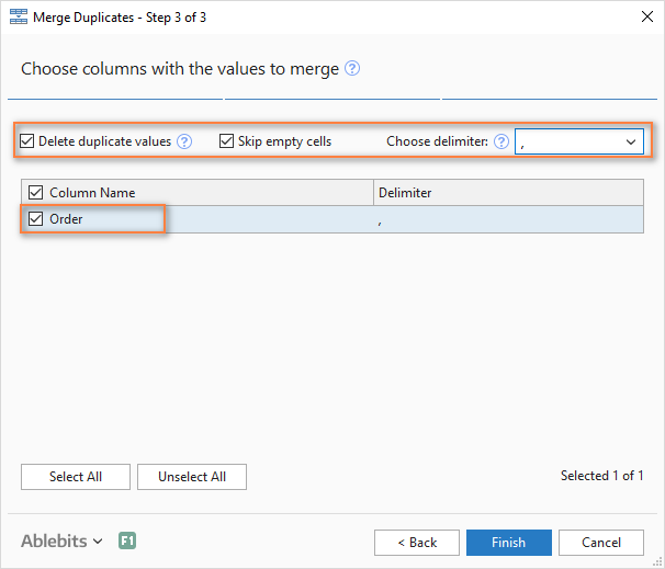
- Choose the columns to merge. In this step, you select the columns whose data you want to combine data and specify the delimiter: semicolon, comma, space, line break, etc.
Two additional options in the upper part of the window let you:
- Delete duplicate values while combining the rows
- Skip empty cells
When done, click the Finish button.
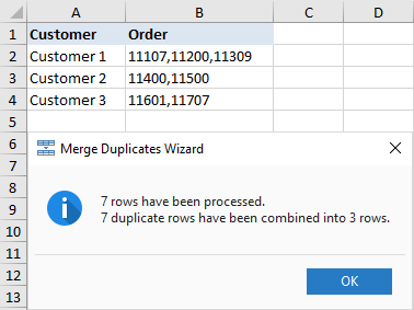
In a moment, all the data from duplicate rows are merged into one row:
How to repeatedly merge blocks of rows into one row
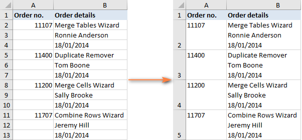
The task: you have an Excel file with information about the recent orders and each order takes 3 lines: product name, customer name and date of purchase. You would like to merge every three rows into one, i.e. repeatedly merge the blocks of three rows.
The following image show what we are looking for:
If there are only few entries to be combined, you can select each 3 rows and merge each block individually using the Merge Cells add-in. But if your worksheet contains hundreds or thousands of records, you will need a faster way:
- Add a helper column to your worksheet, column C in our example. Let's name it BlockID, or whatever name you like.
- Insert the following formula in C2 and then copy it down the column by dragging the fill handle:
=INT((ROW(C2)-2)/3)Where:
- C2 is the topmost cell in which you enter the formula
- 2 is the row where the data starts
- 3 is the number of rows to be combined in each block
This formula adds a unique number to each block of rows, as shown in the screenshot:
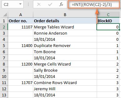
How this formula works: The ROW function extracts the row number of the formula cell, from which you subtract the number of the row where your data start, so that the formula starts counting from zero. For example, our data start in the 2nd row, so we subtract 2. If your data start, say, in row 5, then you will have ROW(C5)-5. After that, you divide the above equation by the number of rows to be merged and use the INT function to round the result down to the nearest integer. - Well, you've done the main part of the work. Now you just need to merge the rows based on the BlockID For this, we will be using the already familiar Merge Duplicates wizard that we utilized for combining duplicate rows:
- In step 2, choose BlockID as the key column.
- In step 3, select all the columns you want to merge and pick line break as the delimiter.
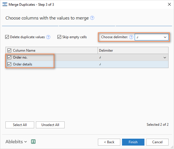
In a moment, you will have the desired result:
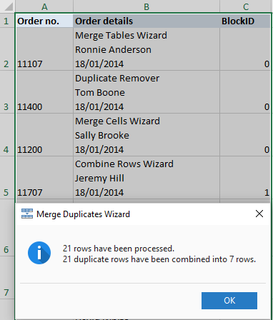
- Delete the Block ID column since you don't need it any longer and you are done! A funny thing is that we've needed 4 steps again, like in the two previous examples :)
How to merge matching rows from 2 Excel tables without copying / pasting
Task: you have two tables with a common column(s) and you need to merge matching rows from those two tables. The tables may be located in the same sheet, in two different spreadsheets or in two different workbooks.
For example, we have sales reports for January and February in two different worksheets and want to combine them into one. Mind you, each table may have a different number of rows and different order of products, therefore simple copy/pasting won't work.
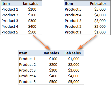
In this case, the Merge Two Tables add-in will work a treat:
- Select any cell in your main table and click the Merge Two Tables button on the Ablebits Data tab, in the Merge group:
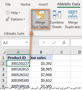
This will run the add-in with your main table preselected, so in the first step of the wizard you simply click Next. - Select the second table, i.e. the lookup table containing the matching rows.
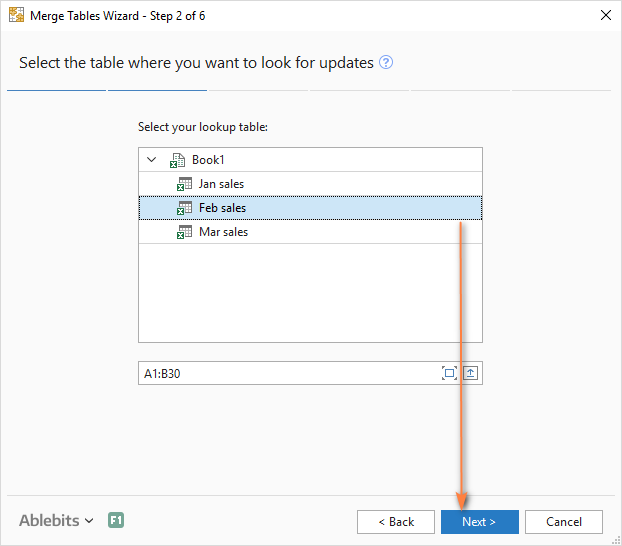
- Choose one or more column columns that exist in both tables. The key columns should contain only unique values, like Product ID in our example.
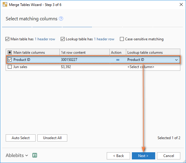
- Optionally, select the columns to update in the main table. In our case, there are no such columns, so we just click Next.
- Choose the columns to add to the main table, Feb sales in our case.
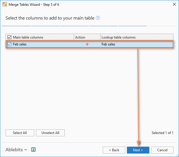
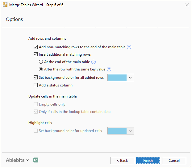
- In the final step, you can select additional options depending on how exactly you want to merge data, and click the Finish button. The screenshot below shows the default settings, that work just fine for us:
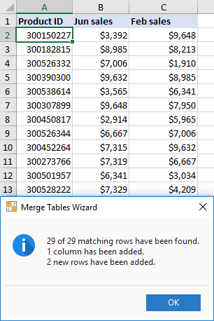
Allow the add-in a few seconds for processing and review the result:
How can I get these merging tools for Excel?
All of the add-ins discussed in this tutorial, plus 70+ other time-saving tools, are included in our Ultimate Suite for Excel. The add-ins work with all versions of Excel 2019, Excel 2016, Excel 2013, Excel 2010 and Excel 2007.
Hopefully, you can now merge rows in your Excel sheets exactly the way you want them. If you have not found a solution for your specific task, just leave a comment and we will try to figure out a way together. Thank you for reading!
Available downloads
Ultimate Suite 14-day fully-functional version (.exe file)
 by
by
113 comments
I am trying to merge all the rows into one ,but i am still losing a lot of values,is their a limit to the tool.
Supposing you have a range of data as below screenshot shown. Now you may need to merge rows of data with the same value in the Fruit column. In this condition, you can apply the Advanced Combine Rows feature of Kutools for Excel to deal with it.
I have a lot of contact information -- the same person is listed in six rows: one of the rows has a phone number but no email, another has an email but no phone. How do I remove the duplicates and keep the phone number and email address in the final unique entry?
Hi there my question is slightly different.
I have numbers lines within a cell, e.g.:
Example A
Example B
Example C
Example D
However, I want them to appear as below:
Example A
Example B
Example C
Example D
So I need to remove the blank lines between the writing but keep the writing on separate lines.
Is there a shortcut for this?
this article is useful......is there any index so that i can search through the blog??
p.s is there a blog on simple formatting and then formatting in more presentable ways
Dear Sir/Mam, How to count the number of rows in merged cells by using formula and not by VBA. For Example, If range A1:A10 is merged then how to get the number of merged rows (i.e. 10) in this range by using only the formula.
Hi,
I need help if i have data in multiple row and i want to combine into multiple column, is it possible in excel?
Example:
Column_A Column_B
AAAA A1
AAAA A2
AAAA A3
The result that i want is:
Column_A Column_B Column_C Column_D
AAAA A1 A2 A3
is it possible?
is there a short way l could merge rows with even gaps into one row. l am using a sheet with several line items which have different row gaps.
Hello,
the simplest and quickest way of combining the rows is using our add-ins: Merge Cells and Combine Rows Wizard.
You can see how they work in the article above and you can also download and install their fully-functional versions to try them out.
how to consolidate the ledger with narration detail in excel
Dear Irina,
I need to merge multiple rows in the same column with one another so that you have all text in one column, and row. Can you please help?
Kind regards
Jan Swart
Dear Jan,
we have just a perfect solution for you - Merge Cells Wizard. With its help, you'll be able to combine multiple cells into one cell/row/column and use any separator to your liking.
You can download and install the trial version of the add-in by using this direct link.
Please find the instructions on how to work with the add-in on its help page.
Hope you'll find the add-in useful!
Hai Irina,
can u please help me?
I have alpbhabets in column A and Assigned values on column B.If I merged some albhabetic letters in C.I need to display the corresponding mergerd values in column D.Is this Poosible?If Yes How?
A B C D
a 1 ac 13 ..................?
b 2
c 3
Thank you
Is there a function in Excel which allows a user simply combine two sheets finding the unique data identifier in both sheets and automatically add the necessary number of additional columns so that all of the data in both sheets would be displayed on the line where the unique identifier is found on each sheet? Seems like there would be a function in Excel to do this easily and automatically without entering any formula.
Irina,
I have two rows, 3 columns with Col A Name, Col B expiration date and Col C email address.
Row 1has the name and email address
Row 2 has the name and expiration date
I need to merge, combine, sort; to obtain the name, expiration date and email address into one row of data
Example:
row 1 Fred fred@fred
row 2 Fred 12/1/2017
Need row Fred 12/1/2017 fred@fred
Hi Charles,
You can use our Combine Rows Wizard add-in to solve this task:
https://www.ablebits.com/excel-combine-rows/index.php
hello dear madam
i have a question
i have a column in excel with many name
and i want to know that how can i marge the same name in column
thanks
Hello Amir,
If your task is to leave only unique names, you can use the Remove Duplicates tool on the Data tab in Excel. If you'd like to merge data from adjacent columns at the same time, then Combine Rows Wizard will help you:
https://www.ablebits.com/excel-combine-rows/index.php
I have a list of contacts to merge. Some rows are for the same person, and have different data than the other rows. One may have an email address, the other the phone number. Sometimes both rows have the same data.
The prior comments are all interesting, but did not have this answer.
Is there a way to merge the rows and retain the best data? I would think I need a VBA macro which allows a dialog box for me to choose the better of the two data points if there is competing data for a column.
This may not be a strictly Excel solution, but do you have any advice for this very common scenario?
Thank you
Hello Curt,
Combine Rows Wizard does exactly what you describe:
https://www.ablebits.com/excel-combine-rows/index.php
You can specify the key columns to know the rows refer to the same record, like the name, and select all other columns for the merge with the option to delete duplicate values; thus you'll get all relevant information on the same row.
If this add-in actually does what it says, I'll most probably purchase it, but I tried the trial version to combine rows and delete duplicates in them but it did not work. I went exactly according to the tutorial above but still it didn't work. After pressing finish, a message comes which says 0 Rows combined, no duplicates found, I don't know what is the problem. Can someone help me with it?
Hello Vikram,
I'm sorry to hear that. Would it be possible for you to describe your task and send a sample spreadsheet to support@ablebits.com? Please also include a link to the post and your comment number. We'll look into this issue.
how can I have Ablebits in my Excel?
Hello Fitz,
You can get both add-ins with Ultimate Suite for Excel, here is a direct link to download a fully-functional 20-day evaluation version:
https://www.ablebits.com/files/get.php?addin=xl-suite
We need to combine the data in excel as follows:
Original Data Expected Data
Name value Name value Combine value for particular Row value
aaaaa 1701 aaaaa 1701 1701,1668,1332,1474
aaaaa 1668 aaaaa 1668 1701,1668,1332,1474
aaaaa 1332 aaaaa 1332 1701,1668,1332,1474
aaaaa 1474 aaaaa 1474 1701,1668,1332,1474
bbbb 1224 bbbb 1224 1224,1758,1512,1812,1382,1234
bbbb 1758 bbbb 1758 1224,1758,1512,1812,1382,1234
bbbb 1512 bbbb 1512 1224,1758,1512,1812,1382,1234
bbbb 1812 bbbb 1812 1224,1758,1512,1812,1382,1234
bbbb 1382 bbbb 1382 1224,1758,1512,1812,1382,1234
bbbb 1234 bbbb 1234 1224,1758,1512,1812,1382,1234
dddd 1641 dddd 1641 1641,1537,1589,1216,1703,1277,1197,1894,1847
dddd 1537 dddd 1537 1641,1537,1589,1216,1703,1277,1197,1894,1847
dddd 1589 dddd 1589 1641,1537,1589,1216,1703,1277,1197,1894,1847
dddd 1216 dddd 1216 1641,1537,1589,1216,1703,1277,1197,1894,1847
dddd 1703 dddd 1703 1641,1537,1589,1216,1703,1277,1197,1894,1847
dddd 1277 dddd 1277 1641,1537,1589,1216,1703,1277,1197,1894,1847
dddd 1197 dddd 1197 1641,1537,1589,1216,1703,1277,1197,1894,1847
dddd 1894 dddd 1894 1641,1537,1589,1216,1703,1277,1197,1894,1847
dddd 1847 dddd 1847 1641,1537,1589,1216,1703,1277,1197,1894,1847
Hi I am interesting in doing exactly the example given in "Merge matching rows from 2 Excel worksheets without copying / pasting" (https://www.ablebits.com/office-addins-blog/merge-rows-excel/#merge-matching-rows). to be brief: Product, Jan sales on 1 sheet and Product, Feb sales on another sheet.
I download the "merge two tables" function but I do not ended up with Product, Jan sales, Feb sales as described. Step4 is actually different. So I am wondering if you guys have updated this function and more important How to do the example because it is exactly what I am looking for?
Thanks a lot for any help
Hello Emmanuelle,
Thank you for contacting us.
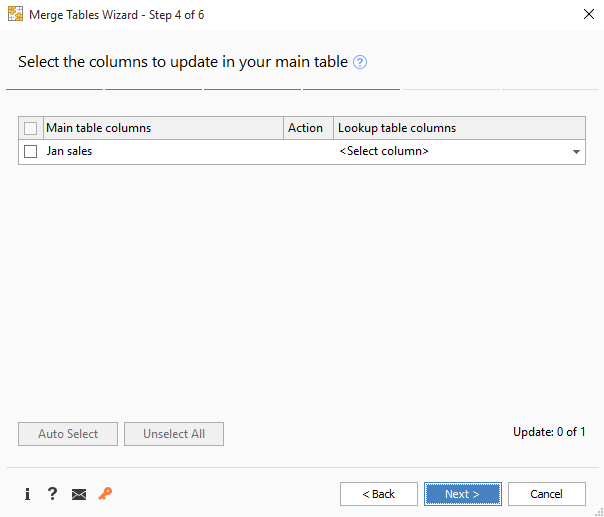
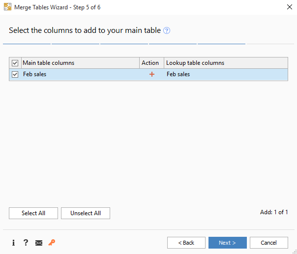
You are right, we slightly changed the add-in, though it has the same functionality. The new version lets you choose the columns to update on step 4, and the columns to add on step 5. If you don't want to update any columns and your task is to add "Feb sales" to your main table, do not select anything on step 4 and click Next:
Once you get to step 5, select Feb Sales:
Choose the necessary additional options on the last step and click Finish to get the desired result.
Hi :)
I've read the part "Repeatedly merge blocks of rows into one row"
How can you make it work if you don't have the first row in your example?
So if you don't have this first row:
| Order no. | Order details | BlockID |
Thanks
Adam
!!!!! And I have only one column which I'd like to be merged this way: Merging 1-18, Merging 19-36, Merging 37-54. (and do not delete the text: "blablabla".
So I'd like to merge every 18 rows. (and do not delete the text: "blablabla".
From this:
_________________
1.___blablabla___
2._______________
3._______________
4._______________
5._______________
6._______________
7._______________
8._______________
9._______________
10.______________
11.______________
12.______________
13.______________
14.______________
15.______________
16.______________
17.______________
18.______________
19.__blablabla___
20.______________
21.______________
22.______________
23.______________
24.______________
25.______________
26.______________
27.______________
28.______________
29.______________
30.______________
31.______________
32.______________
33.______________
34.______________
35.______________
36.______________
37.__blablabla___
38.______________
39.______________
40.______________
41.______________
42.______________
43.______________
44.______________
45.______________
46.______________
47.______________
48.______________
49.______________
50.______________
51.______________
52.______________
53.______________
54.______________
It should be like this:
_________________
1. |
2. |
3. |
4. |
5. |
6. |
7. |
8. |
9. blablabla |
10. |
11. |
12. |
13. |
14. |
15. |
16. |
17. |
18.______________|
19. |
20. |
21. |
22. |
23. |
24. |
25. |
26. |
27. |
28. blablabla |
29. |
30. |
31. |
32. |
33. |
34. |
35. |
36.______________|
37. |
38. |
39. |
40. |
41. |
42. |
43. |
44. |
45. |
46. blablabla |
47. |
48. |
49. |
50. |
51. |
52. |
53. |
54.______________|
55. |
56. |
57. |
and so on...
Hello Adam,
Thank you for sending the example to us.
Since formulas work with values, you can merge every n cells only with the help of VBA. One of our developers wrote the code for you, please follow these steps:
- Open your Excel file and select the column with the values you'd like to merge (column A in your sample file);
- Press Alt+F11 on your keyboard;
- Double-click the sheet name in the list and paste this code:
Sub merge()
Dim reg As Range
Dim start As Range
Dim startVal As String
Dim size As Integer
Set reg = Application.Selection
size = reg.Cells.Count
startVal = reg.Cells(size, 1).Value
Set start = reg.Cells(size, 1)
For i = size To 1 Step -1
If startVal <> reg.Cells(i, 1).Value Then
Application.ActiveSheet.Cells.Range(reg.Cells(i, 1), start).merge
If i <> 1 Then
Set start = reg.Cells(i - 1, 1)
startVal = reg.Cells(i - 1, 1).Value
End If
End If
Next
End Sub
- Click Run.
This should do the trick.
Hi,
I want to merge 3 cells into 2. Please tell me if it is possible.
Thank You
Hello Rishabh,
Could you please provide an example of the data you have in three cells and of what you want to get in two cells as a result? You can send a sample spreadsheet to support@ablebits.com.
nice
Pls suggest how do I concatenate for 5000 cells ?
Hello,
Could you please describe the way you want to concatenate 5000 cells? If possible, please send a sample spreadsheet to support@ablebits.com
I have 3 rows as AB0U-RFW-010-9012-01 AB0U-RFW-010-9012-02, AB0U-RFW-010-9012-03, AB0U-RFW-010-9012-04
i want only one entry to show AB0U-RFW-010-9012-01~04 can you help how to getthis
how i can change the data 03 or 4 row to one
Hi plz help me for moving data to other file without loss
Bonjour! I hope you will be able to help me! I have an Excel sheet containing column A, listing natural medicinal substances. Then columns B to AA have headers indicating the possible medicinal uses of said substances. There are 26 uses and I put "X"s in the column(s) that correspond to each substance's uses.
To make a long story short, at first I had one excel spreadsheet for each use of my substances, and I now want to combine all the data in one larger spreadsheet. BUT, since each substance has multiple uses, I end up with, for example, 4 rows for "Tansy" (Ex. A 21, 22, 23, 24), and in each row, an X appears in the column corresponding to one use of the herb (Ex:B:21, C:22, J:23 and Y:24). What I would like to do is to combine the 4 Tansy rows into one (ex. row 21), where I would have B:32, C:21, J:21 and Y:21.
I hope I managed to be clear, and I thank you very much in advance for any help you could provide in letting me know is your Wizards could solve my problem! IM
Hello Isabelle,
It sounds like you can use Combine Rows Wizard for your task:
- Select all your data on step 1 and choose to create a backup copy just in case;
- Select column A with the substances on step 2;
- Use the top check-box to select all columns with the uses on step 3, and select the options to "Delete duplicate values" and "Skip empty cells". As you have the same "X"s in all cells, it doesn't matter what delimiter you leave in the field.
- Click Finish
If you have any difficulties, please send a sample worksheet to support@ablebits.com, we'll do our best to assist you.
Can anyone help me out on how to repeatedly merge blocks of uneven rows into one row.
I have very large data with uneven blocks of row.
I have something like the table below
Name Reported Date+"" Summary*"" Notes""
Istifanus 5/4/2015 8:08 2-IT Incident Report - Hardware - Dear Team,
abcd
efgh
kjil
Jane 5/4/2015 8:17 2-IT Incident Report - Hardware - Good morning,
port
Newman
Anderson
Caleb 5/4/2015 8:27 2-IT Incident Report - Hardware - Stevedores
I want to merge the Notes into one cell against the other contents of the first row.
Thank you for your help
Dear All, Am trying to merge multiple rows in a particular column without affecting the contents of other columns.
I'll appreciate if anyone have an idea on how to go about this
Firstly, great article and very well explained!
Secondly, I receive client databases in excel files. However, while we want to receive the data like this:
Column 1 Column 2 Column 3 Column 4
John Smith 10 Smith St John@gmail.com
Instead we get the data like this:
Column 1 Column 2 Column 3 Column 4
John Smith 10 Smith St John@gmail.com Nothing Nothing Nothing
or this:
Column 1 Column 2 Column 3 Column 4
John,Smith,10 Smith St,John@gmail.com Nothing Nothing Nothing
Is there a way to write up a script or some way to reformat the data to get the format we want - which is the first example?
I am trying to bring an output over to another cell for a schedule that I am creating my worksheet is broken down into 15 minute intervals and I am trying to get the lunch to cover an hour
my current formula is as follows
=IF($B9>G$1,"FREE",IF($F9<G$1,"FREE",IF($C9=G$1,"BREAK",IF($D9=G$1,"lunch",IF($E9=G$1,"BREAK","DL")))))
I can only get the if summary to output lunch to that one 15 minute cell does anyone know how I can add it to multiple cells without changing my data table or how I can merge multiple cells with my formula
Hello Andrew,
I am sorry, it is difficult to recommend you something without seeing your data. For us to be able to assist you better, please post a small sample workbook with your data on our forums. Our support team will try to help.
okay I will do that.. but basically what I would like to do is in my formula tell lunch to consume 4 cells instead of just one by copying over 4 times without creating an endless cycle or tell the the "lunch" to merge multiple cells when during that time slot
I have an inventory report that shows the cost when we purchased items. It first lists the item number and description, and then on another line it shows the date, qty, cost. Some items have just one purchase date, ie one row, and others have up to 5 rows. The items with multiple rows have a subtotal, the ones with one row do not. I want to get the part number and description on the same line(s) as the purchase date information. How do I do that?
More detail:
cell A2 and B2 have the item# and description.
Cell B3 C3, D3, E3 have the purchase date, item cost, and qty. and extended cost.
But sometimes there will also be a Cell B4, C4, D4 and E4 with another purchase date, cost and qty. And then this would be followed with a subtotal of the qty and cost in row 5.
I need to get the Item# and Description to show up on all the lines for that part.
HELP!???
Hello Tommy,
I am sorry, but there is no way to fulfill your task using formulas. If your data are more or less sorted, a special VBA macro should help. You can ask for it on http://www.mrexcel.com or http://www.excelforum.com
If your data are distorted, you’d better hire freelancers who sort your data manually or write a macro.
Hi
How do you link an excel populated data sheet(A) to another data sheet(B) but manage to keep the information lock to dates when data is combined in data sheet(B).
Thank You
I have an online order system that gives me an excel sheet of individual items placed in an order. I want to merge the items and quantity based on each order. Is this possible with your program?
Example:
Order Item Quantity
100 Plates 500
100 Shoes 2
101 Phones 1
101 Paper 3
I would like it to look like this (or similar):
Order Item
100 Plates - 100, Shoes - 2
101 Phones - 1, Paper - 3
I tried INT((ROW(C2)-2/3)) to combine multiple rows in my spreadsheet and I did get a value of 1 for C2, but I cannot find the block id or combine row wizard in Excel 2007.
Thanks,
Shana
I have a very lengthy spreadsheet, and I need to sort everything into alphabetical order by name in column "A", but each cell in column "A" has specific data in columns "B" thru "G" linked to it. Is there a way I can sort alphabetically without mixing up all the other data. My only thought was to merge each row entirely, and then sort via alphabetical order than un-merge all rows. Is there an easier way?
Nevermind.
Am not sure what I need is covered? I have two equal length adjacent columns, both containing text. I need to merge the text in column 1 with the text in column 2, into a single column (say 3) with no loss of data.
For example,
1 2 3
A X A,X
B Y BECOMES B,Y
C Z C,Z
. . .
. . .
Hello Peter,
Here's the formula:
=IF(AND(ISNUMBER(A1),ISNUMBER(B1)),A1+B1,A1&","&B1)
Spot on!
Thanks,
P
Hello Svetlana,
Is there any formula to merge multiple empty cells in a column?
Thank you
Hi,
I want to merge the rows. but in the content some of the rows are blanks. i tried the concatenate formula like this(=A1&","A2) . Its not working. Tell me how to merge the rows with comma if there are blank rows inbetween the content.
Hello Mike,
Sorry, I do not exactly understand the task. If you can send a sample workbook with your data to support@ablebits.com and include the result you want to get, our support team will try to help.
Hi,
Is there a way to use the combine rows and have the program actually write out all the columns instead of entering data in a column separated by semicolons or commas? I want the duplicate data actually expanded across columns:
Sample
A B 32 25 Y N
A C 32 22 N Y
Combined
A B C 32 32 35 22 Y N N Y
I love the program, it is fantastic but I need to expand the results and not sure how to do that.
Thanks,
Gene
Hello Gene,
If you have simple data (without commas), the following solution might work for you:
1 Run Combine Rows Wizard to merge the data and choose a semicolon as the separator.
2 Save the resulting worksheet as a .csv file. For more details, please see this article:
https://www.ablebits.com/office-addins-blog/convert-excel-csv/
3 Open the .csv file in Notepad and replace all semicolons with commas. Save the file.
4 Open the .csv file in Excel, see here for full details:
https://www.ablebits.com/office-addins-blog/convert-csv-excel/
Hi Svetlana,
Hope you are doing good.
Quick question.
Lets say I have:
firstname lastname email
abc dec test@gmail.com
123 456 123456@gmail.com
When filling in the data, at times, the email is firstnamelastname@<email.com.
I would like a way that when this is the case, I use a shortcut and firstnamelastname is automatically pasted in the 3rd column.
Now this has to be a shortcut cause not always, this is the case.
I hope you understood my query. Is this possible in any manner?
Kind Regards,
Hem
Hi Hem,
If my understanding is correct, it is not possible to fulfill your task using formulas. Most likely you need a small VBA macro.
Hi there, how to I undo the merged cells?
Hello Sumen,
It depends on how the cells were merged. If you have just merged them, you can use the standard Excel Undo feature (Ctrl+Z). Our merging add-ins create a backup copy of your worksheet before merging the data. In other cases, I'm afraid, Undo is not possible.
I am having the list as mentioned below and i want the result which is mentioned.
please help by provinding the solution as mentioned in name coloum is change day by day i expecting the formula from where he automaticaly give me the result name of the customer which is present in name column.
Name code amount
Abc 123 2
DEF 456 3
GHF 458 4
KLM 741 5
NMR 351 6
DEF 456 7
KLM 741 8
MNP 3425 9
NMR 351 10
MNP 3425 11
JKL 7538 12
Abc 123 13
DEF 456 14
GHF 458 15
GHF 458 16
DEF 456 17
DEN 753 18
I want the Result to be like mentioned below by using the formaulas
Name Code Amount
Abc 123 15
GHF 458 35
DEF 456 41
KLM 741 13
NMR 351 16
MNP 3425 20
JKL 7538 12
DEN 753 18
I believe the following solutions will work:
Solution 1:
- Sort your table by the Name column.
- Go to Data > Outline and click on Subtotal.
- Specify the following settings:
At each change in: Name
Use function: Sum
Add subtotal to: Amount
- Click OK and then press Number 2 in the upper left-hand corner of your worksheet to get the sum by name.
For more information about using subtotals in Microsoft Excel, please see:
https://www.ablebits.com/office-addins-blog/subtotal-excel-insert-use-remove/
Solution 2:
- Insert a pivot table (select your table and go to Insert > Tables > PivotTable).
- Choose to insert the PivotTable report onto a new worksheet and click OK.
- In the PivotTable Fields pane, drag and drop the Names column to the Rows section and the Amount column to the Values section.
You will get the same result.
Solution 3:
- Copy your table to another worksheet
- Go to Data > Remove duplicates to delete duplicated names.
- Type the following formula in the Amount column:
=SUMIF('V3 - source'!A2:A18,A2,'V3 - source'!C2:C18)
Where 'V3 - source'!A2:A18 is the reference to the Names column of your source data, 'V3 - source'!C2:C18 – the reference to the Amount column.
You can download the workbook with all 3 solutions using the below link:
https://cdn.ablebits.com/_img-blog/_comments/jhon%20-%20119.235.57.75%20-%20sumif.xlsx
I am having a 5000 customer in Column "A" and In column "A' most of the customer is repeated Now i want the formulas from which i will check the names of the customer which is present in this column.
Hello John,
There exist a number of solutions depending on what exactly result you are trying to achieve.
If you want to highlight all duplicates in a column, please see this article:
https://www.ablebits.com/office-addins-blog/how-to-highlight-duplicates-excel/
To highlight duplicate entries between 2 columns, see the "Compare 2 columns for duplicates" example on this page:
https://www.ablebits.com/office-addins-blog/excel-conditional-formatting-formulas/
If you want to merge the duplicate rows into one, check out the Combine Duplicated Rows add-in:
https://www.ablebits.com/excel-combine-rows/index.php
Thank you so much for this!! I was pulling my hair out trying to merge address data into one cell so that it would be more usable in a Mail merge in Microsoft Office. You saved my day!!! Thank you, thank you, thank you!!!
let's say I have 2 rows of the exact same data, except for ONE cell in each column.
For an example, let's make the headers: a. Customer Name, b. Customer ID, c. Customer Address, and d. Amount Paid.
Now rows 1 & 2 are the exact same customer, except in row 1 column d the dollar amount is $500, and in row 2 the dollar amount is $300.
Is there a way to quickly consolidate into a single line, with the dollar amount in column d the sum of the previous entries? (i.e. $800)?
Hello Harold,
You can do this in 2 ways:
1. Using Subtotal. Sort your table by Customer ID and then apply subtotal in this way: At each change in "Customer ID", use function "Sum", add subtotal to column "Amount Paid". Please see this article for more details: Using Subtotals in Microsoft Excel
2. Using a pivot table.
Hi Swetlana
I can not find the menu and i want to help you on urgent basses so kindly help me.
Regards
Mukesh Walia
Hello Mukesh,
I am sorry, I do not exactly understand the problem. Do you mean you do not see the add-in's menu in Excel after installation? Anyway, you can reach our support team at support@ablebits.com and we will promptly respond and fix the issue.
I tried out this merging tool for the past two days and I like it a lot, but I run into problems, as soon as I try to combine a sheet that just contains text and number data with a sheet that has a date column. Is there something that has to be considered when doing this? I tried every possible combination, but it just does not seem, that my merged values are ever correct...
Hello Bridget,
Thank you for your interest in our merging add-in for Excel, I am really glad to know you like it!
I'm afraid we cannot determine the exact cause of the problem without seeing your data. Can you please send me your workbook (or just a sample of data) at support@ablebits.com and describe the result you are trying to achieve? I will do my best to help.
Can I use this tool if I need to use the contents 2 columns ?
Hi Gayle,
Of course, you can use one of the tools described in the article, Merge Cells add-in, to combine the contents of 2 columns. You can find the detailed description with screenshots here.
Hey Friend If u are still here so please tell me how to Merge or combine two column without losing data...like 1 have numbers in A1 and AW1,AX1 both had merged.i want copy A1 number to AW1,AX1...i Have a Very Big Spreadsheet..is it Possible or i ahve to do Manually...please Reply Fast..Thanks...
Hi Akbar,
You can find several solutions in this article: How to merge two columns in Excel without losing data. Hope you will find them helpful.